1
 2
 3
 4
 5
 6
 7
 8
 9
10
11
12
13
14
15
16
17
18
19
20
21
22
23
24
25
26
27
28
29
30
31
32
33
34
35
36
37
38
39
40
41
42
43
44
45
46
47
48
49
50
51
52
53
54
55
56
57
58
59
60
61
62
63
64
65
66
67
68
69
70
71
72
73
74
75
76
77
78
79
80
81
82
83
84
85
86
87
88
89
90
91
92
93
94
95
96
97
98
99
100
101
102
103
104
105
106
107
108
109
110
111
112
113
114
115
116
117
118
119
120
121
122
123
124
125
126
127
128
129
130
131
132
133
134
135
136
137
138
139
140
141
142
143
144
145
146
147
148
149
150
151
152
153
154
155
156
157
158
159
160
161
162
163
164
165
166
167
168
169
170
171
172
173
174
175
176
177
178
179
180
181
182
183
184
185
186
187
188
189
190
191
192
193
194
195
196
197
198
199
200
201
202
203
204
205
206
207
208
209
210
211
212
213
214
215
216
217
218
219
220
221
222
223
224
225
226
227
228
229
230
231
232
233
234
235
236
237
238
239
240
241
242
243
244
245
246
247
248
249
250
251
252
253
254
255
256
257
258
259
260
261
262
263
264
265
266
267
268
269
270
271
272
273
274
275
276
277
278
279
280
281
282
283
284
285
286
287
288
289
290
291
292
293
294
295
296
297
298
299
300
301
302
303
304
305
|
rm(list = ls())
options(stringsAsFactors = FALSE)
library(tidyverse)
#install.packages("WGCNA")
library(WGCNA)
setwd('C:/Users/30521/Desktop/R自学/GEO-analysis/WGCNA/GSE84844')#设置工作路径
load('GSE84844.rda')

# 1.数据准备####
# 转置,注意!!!:exp类型一定要提前转为数字
# exp <- exp %>% mutate(across(everything(), as.numeric))
exp <- as.data.frame(t(exp))
#输入的基因:可以是全部基因、或者高变基因、也可以是差异基因,建议至少至少2000以上
#样本:15对15以上

# 1.1 选取高变基因,var方差前百分之
# apply用于处理每列基因的方差,'2'指按列处理,'1'指按行处理
vars_res <- apply(exp,2,var)
# 计算百分位数截止值
per_res <- quantile(vars_res, probs = seq(0, 1, 0.25)) # quantile生成分位数
# 选取方差位于前25%的基因
per_gene <- exp[, which(vars_res > per_res[4])]
datExpr0 <- data.matrix(per_gene)

# 1.2 选取高变基因,绝对偏差中位数排名前5000的基因
# mad_res <- apply(exp, 2, mad, na.rm = TRUE)
# mad_gene <- exp[, order(mad_res, decreasing = TRUE)[1:5000], drop = FALSE]
# datExpr0 <- data.matrix(mad_gene)

# 2.数据检查####
#检查样本和基因是否ok
gsg = goodSamplesGenes(datExpr0, verbose = 3)
gsg$allOK

#如果没有达标就需要筛选,[1] TRUE 也能运行,不影响结果
if (!gsg$allOK){
  # Optionally, print the gene and sample names that were removed:
  if (sum(!gsg$goodGenes)>0)
    printFlush(paste("Removing genes:", paste(names(datExpr0)[!gsg$goodGenes], collapse = ", ")));
  if (sum(!gsg$goodSamples)>0)
    printFlush(paste("Removing samples:", paste(rownames(datExpr0)[!gsg$goodSamples], collapse = ", ")));
  # Remove the offending genes and samples from the data:
  datExpr0 = datExpr0[gsg$goodSamples, gsg$goodGenes]
}

#进行样本聚类
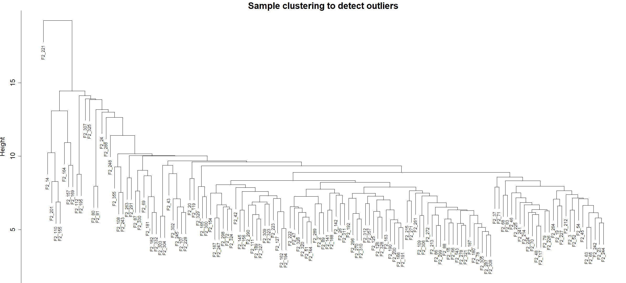
sampleTree = hclust(dist(datExpr0), method = "average")
par(cex = 0.6)
par(mar = c(0,4,2,0))
plot(sampleTree)
plot(sampleTree, main = "Sample clustering to detect outliers", sub="", xlab="", cex.lab = 1.5, cex.axis = 1.5, cex.main = 2)
#剪切线
abline(h = 70, col = "red")

#切除未聚类的样本,看的是样本的合并高度
clust = cutreeStatic(sampleTree, cutHeight = 70, minSize = 10)#注意:cutHeight = 这里才是真正切割
table(clust)
keepSamples = (clust==1)
#注意查看切割数量0有多少 1有多少
datExpr0 = datExpr0[keepSamples, ]


#表型数据分组
table(rt)
# 根据具体临床数据,control列的control对应为1,pSS对应为0;同样地运用于建立的pSS列
traitData <- data.frame(control=c(rep(1,30),rep(0,30)),
                        pSS=c(rep(0,30),rep(1,30)))
row.names(traitData) <- rownames(exp)

sameSample <- intersect(rownames(datExpr0), rownames(traitData))
datExpr <- datExpr0[sameSample,]
datTraits <- traitData[sameSample,]

#去除后再聚类
sampleTree2 = hclust(dist(datExpr), method = "average")
plot(sampleTree2)
#标记颜色
traitColors = numbers2colors(datTraits, signed = FALSE)
# 3.第一部分样本可视化作图####
# 完成样本与表型的聚类
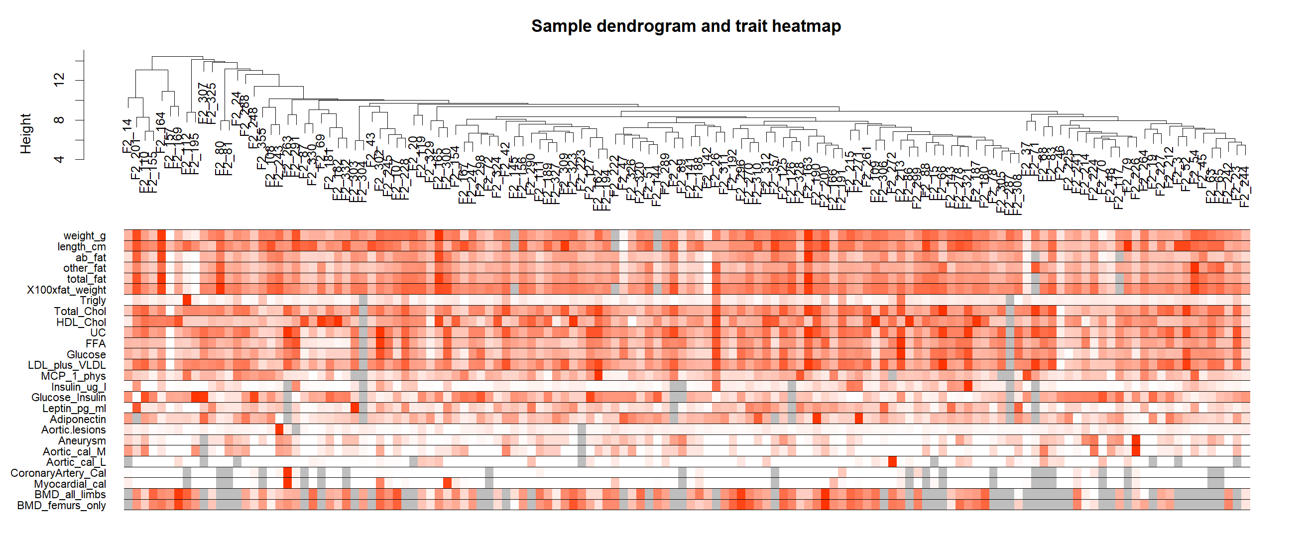
plotDendroAndColors(sampleTree2, traitColors,
                    groupLabels = names(datTraits),
                    main = "Sample dendrogram and trait heatmap")
save(datExpr, datTraits, file = "WGCNA_data1.rda")

# 4.网络构建####
rm(list = ls())
load(file = "WGCNA_data1.rda")
#power值散点图
allowWGCNAThreads()   #多线程工作
powers = c(c(1:10), seq(from = 12, to=20, by=2)) #幂指数范围1到20
powers
sft = pickSoftThreshold(datExpr, powerVector = powers, verbose = 5)
sft

#作图
sizeGrWindow(9, 5)
par(mfrow = c(1,2))
cex1 = 0.9
#拟合指数与power值散点图,确保散点在0.8以上,最好0.9以上
plot(sft$fitIndices[,1], -sign(sft$fitIndices[,3])*sft$fitIndices[,2],
     xlab="Soft Threshold (power)",ylab="Scale Free Topology Model Fit,signed R^2",type="n",
     main = paste("Scale independence"));
text(sft$fitIndices[,1], -sign(sft$fitIndices[,3])*sft$fitIndices[,2],
     labels=powers,cex=cex1,col="red");
abline(h=0.90,col="red") #根据自己选择修改,如0.9则不变
###平均连通性与power值散点图
plot(sft$fitIndices[,1], sft$fitIndices[,5],
     xlab="Soft Threshold (power)",ylab="Mean Connectivity", type="n",
     main = paste("Mean connectivity"))
text(sft$fitIndices[,1], sft$fitIndices[,5], labels=powers, cex=cex1,col="red")

#自动计算softPower,自动评估软阈值
softPower <- sft$powerEstimate
softPower
#查看最佳softPower值
#选择power
softPower = 6
adjacency = adjacency(datExpr, power = softPower)

#TOM矩阵
TOM = TOMsimilarity(adjacency);
dissTOM = 1-TOM
#基因聚类
geneTree = hclust(as.dist(dissTOM), method = "average")
plot(geneTree, xlab="", sub="", main = "Gene clustering on TOM-based dissimilarity",
     labels = FALSE, hang = 0.04)
##动态剪切模块识别
minModuleSize = 30  #最小模块基因数
dynamicMods = cutreeDynamic(dendro = geneTree, distM = dissTOM,
                            deepSplit = 2, pamRespectsDendro = FALSE,
                            minClusterSize = minModuleSize);
table(dynamicMods)
#标记颜色
dynamicColors = labels2colors(dynamicMods)
table(dynamicColors)
#5.第二部分基因聚类作图####
plotDendroAndColors(geneTree, dynamicColors, "Dynamic Tree Cut",
                    dendroLabels = FALSE, hang = 0.03,
                    addGuide = TRUE, guideHang = 0.05,
                    main = "Gene dendrogram and module colors")

#6.相似模块聚类####
MEList = moduleEigengenes(datExpr, colors = dynamicColors)
MEs = MEList$eigengenes
MEDiss = 1-cor(MEs);
METree = hclust(as.dist(MEDiss), method = "average")
sizeGrWindow(7, 6)
plot(METree, main = "Clustering of module eigengenes",
     xlab = "", sub = "")

#剪切高度,0.25标识相异性(代表75%以上相似性模块合并)及MEDissThres越小代表要求相似性越高,最终模块越多
MEDissThres = 0.25
abline(h=MEDissThres, col = "red")
#相似模块合并(也可不做,根据结果调整)
merge = mergeCloseModules(datExpr, dynamicColors,cutHeight = MEDissThres, verbose = 3)
mergedColors = merge$colors
mergedMEs = merge$newMEs
plotDendroAndColors(geneTree, mergedColors,"Dynamic Tree Cut",
                    dendroLabels = FALSE, hang = 0.03,
                    addGuide = TRUE, guideHang = 0.05,
                    main = "Gene dendrogram and module colors")
moduleColors = mergedColors
table(moduleColors)
colorOrder = c("grey", standardColors(50))
moduleLabels = match(moduleColors, colorOrder)-1
MEs = mergedMEs
save(MEs, moduleLabels, moduleColors, geneTree, file = "WGCNA_data2.rda")

#7.第三部分模块与特征热图####
#模块与表型数据热图
rm(list=ls())
load('WGCNA_data1.rda')
load('WGCNA_data2.rda')
nGenes = ncol(datExpr)
nSamples = nrow(datExpr)
moduleTraitCor = cor(MEs, datTraits, use = "p")
moduleTraitPvalue = corPvalueStudent(moduleTraitCor, nSamples)
#热图展示
textMatrix = paste(signif(moduleTraitCor, 2), "\n(",
                   signif(moduleTraitPvalue, 1), ")", sep = "")
dim(textMatrix) = dim(moduleTraitCor)
sizeGrWindow(10,6)
par(mar = c(6, 8.5, 3, 3))
labeledHeatmap(Matrix = moduleTraitCor,
               xLabels = names(datTraits),
               yLabels = names(MEs),
               ySymbols = names(MEs),
               colorLabels = FALSE,
               colors = blueWhiteRed(50), #greenWhiteRed
               textMatrix = textMatrix,
               cex.lab.y = 0.5,
               cex.lab.x = 0.5,
               setStdMargins = FALSE,
               cex.text = 0.5,
               zlim = c(-1,1),
               main = paste("Module-trait relationships"))

#模块选择相关性0.4以上,P<0.05
#结果不好,调节高变基因,如25%至50%

# 8.模块提取####
modNames = substring(names(MEs), 3)

geneModuleMembership = as.data.frame(cor(datExpr, MEs, use = "p"))
MMPvalue = as.data.frame(corPvalueStudent(as.matrix(geneModuleMembership), nSamples))

names(geneModuleMembership) = paste("MM", modNames, sep="")
names(MMPvalue) = paste("p.MM", modNames, sep="")
#完成基因模热图

#进行模块基因输出
# 基因与表型的相关性
traitNames=names(datTraits)
geneTraitSignificance = as.data.frame(cor(datExpr, datTraits, use = "p"))
GSPvalue = as.data.frame(corPvalueStudent(as.matrix(geneTraitSignificance), nSamples))
names(geneTraitSignificance) = paste("GS.", traitNames, sep="")
names(GSPvalue) = paste("p.GS.", traitNames, sep="")

#9.批量输出散点图####
for (trait in traitNames){
  traitColumn=match(trait,traitNames)
  for (module in modNames){
    column = match(module, modNames)
    moduleGenes = moduleColors==module
    if (nrow(geneModuleMembership[moduleGenes,]) > 1){
      outPdf=paste(trait, "_", module,".pdf",sep="")
      pdf(file=outPdf,width=7,height=7)
      par(mfrow = c(1,1))
      verboseScatterplot(abs(geneModuleMembership[moduleGenes, column]),
                         abs(geneTraitSignificance[moduleGenes, traitColumn]),
                         xlab = paste("Module Membership in", module, "module"),
                         ylab = paste("Gene significance for ",trait),
                         main = paste("Module membership vs. gene significance\n"),
                         cex.main = 1.2, cex.lab = 1.2, cex.axis = 1.2, col = module)
      abline(v=0.8,h=0.5,col="red")
      dev.off()
    }
  }
}

#10.批量输出模块基因####
for (mod in 1:nrow(table(moduleColors)))
{
  modules = names(table(moduleColors))[mod]
  probes = colnames(datExpr)
  inModule = (moduleColors == modules)
  modGenes = probes[inModule]
  write.table(modGenes, file =paste0(modules,".txt"),sep="\t",row.names=F,col.names=F,quote=F)
}

#11.其他补充图####
rm(list=ls())
load('WGCNA_data1.rda')
load('WGCNA_data2.rda')
nGenes = ncol(datExpr)
nSamples = nrow(datExpr)
#11.1 TOM聚类图####
dissTOM = 1-TOMsimilarityFromExpr(datExpr, power = 6);#power与之前保持一致
#增加强度
plotTOM = dissTOM^7;
#对角线设置为NA
diag(plotTOM) = NA;
#绘图(十分缓慢,建议进行nSelect挑选)
sizeGrWindow(9,9)
TOMplot(plotTOM, geneTree, moduleColors, main = "Network heatmap plot, all genes")

#挑选基因,快速作图
nSelect = 400
set.seed(10);
select = sample(nGenes, size = nSelect);
selectTOM = dissTOM[select, select];
selectTree = hclust(as.dist(selectTOM), method = "average")
selectColors = moduleColors[select];
sizeGrWindow(9,9)
plotDiss = selectTOM^7;
diag(plotDiss) = NA;
TOMplot(plotDiss, selectTree, selectColors, main = "Network heatmap plot, selected genes")

#11.2 特征模块热图####
rm(list=ls())
load('WGCNA_data1.rda')
load('WGCNA_data2.rda')
#重新计算模块特征基因
MEs = moduleEigengenes(datExpr, moduleColors)$eigengenes
#提取特征
Traits = as.data.frame(datTraits$pSS); #选择特征为pSS
names(Traits) = "Traits"
#将特征添加到现有模块特征基因中
MET = orderMEs(cbind(MEs, Traits))
#绘制特征基因与性状之间的关系图
par(cex = 1)
plotEigengeneNetworks(MET, "", marDendro = c(0,4,1,2), marHeatmap = c(3,4,1,2), cex.lab = 0.8, xLabelsAngle
                      = 90)

#绘制树状图
sizeGrWindow(6,6);
par(cex = 1.0)
plotEigengeneNetworks(MET, "Eigengene dendrogram", marDendro = c(0,4,2,0),
                      plotHeatmaps = FALSE)
#绘制热图矩阵
par(cex = 1.0)
plotEigengeneNetworks(MET, "Eigengene adjacency heatmap", marHeatmap = c(3,4,2,2),
                      plotDendrograms = FALSE, xLabelsAngle = 90)
#WGCNA结束
|