R语言中绘图可以选取自带的基础绘图系统plot()，也可以选择ggplot2包。前者像“命令式”作画，一步步下达指令，在画布上添加元素；后者像“声明式”设计，基于“图形语法”，用“图层”叠加的方式构建图形。

基础内容

绘图模板如下：

1
2
3
4
5
6
7
8


ggplot(data = 数据集, mapping = aes(映射规则)) +
  geom_xxx(图层参数, stat = 统计变换, position = 位置调整) + # 几何图层
  scale_xxx(标度参数) + # 坐标轴/颜色/形状标度
  coord_xxx() + # 坐标系
  facet_xxx() + # 分面
  labs() + # 标题、坐标轴标签
  guides() + # 图例精细调整
  theme() # 全局美化主题

geom_xxx（绘图类型）:

`geom_point()` 散点图	`geom_smooth()` 拟合曲线（线性 /loess 平滑，自带置信区间）	`geom_line()` 折线图（x 轴数值从小到大排序）	`geom_path()` 连线（从上到下的原始行顺序）
`geom_boxplot()` 箱线图（分组分布）	`geom_violin()` 小提琴图	`geom_jitter()` 抖动散点（解决点重叠）	`geom_histogram()` 直方图（连续变量分布）
`geom_density()` 密度曲线	`geom_col()` 柱状图（y数值作为柱子高度）	`geom_bar()` 计数柱状图（统计 x 频数）	`geom_text()`/`geom_label()` 文字标签
`geom_errorbar()` 误差棒	`geom_hline()`/`geom_vline()` 水平 / 垂直参考线	`geom_ribbon()` 画两条 y 曲线之间填充的带状区域	`geom_rug()` 边缘地毯图(一种一维散点图)

stat 统计变换：geom 底层自带统计计算，可手动修改stat参数

`stat="count"`	计数（geom_bar 默认）
`stat="identity"`	直接使用原始 y 值（geom_col 默认）
`stat="smooth"`	拟合平滑曲线（geom_smooth）
`stat="bin"`	分箱统计（直方图）

position 位置调整：解决重叠

`position = "identity"`	默认，不偏移
`position = "dodge"`	分组并列柱状图
`position = "stack"`	堆叠柱状图
`position = "fill"`	百分比堆叠柱状
`position = "jitter"`	点抖动防重叠

scale标度：负责数据→视觉属性转换，同时生成坐标轴刻度、图例，命名规则为scale_视觉属性_类型

`scale_x_continuous()`/`scale_y_continuous()`	连续轴（对数`trans="log10"`、调整范围 limits）
`scale_x_discrete()`	分类 x 轴（修改标签、调整顺序）
`scale_color_manual()`/`scale_fill_manual()`	手动自定义颜色向量
`scale_color_brewer()`	RColorBrewer 配色
`scale_color_viridis_c()`	连续渐变配色
`scale_size()`、`scale_shape_manual()`	大小 / 形状标度

coord 坐标系：

`coord_cartesian()`	默认直角坐标
`coord_flip()`	xy 轴翻转，横向柱状图
`coord_polar()`	极坐标（饼图、雷达图）
`coord_log10()`	对数坐标轴
`coord_fixed()`	固定 xy 轴比例（等比例散点图）

Facet 分面（多子图）：按分类变量自动拆分图表，无需循环绘图

`facet_wrap(~变量)`	一维分面，自动换行
`facet_grid(行变量 ~ 列变量)`	二维网格分面

主题系统美化：

1）内置完整主题：

`theme_bw()`	白底 + 浅灰色网格线，带黑色边框
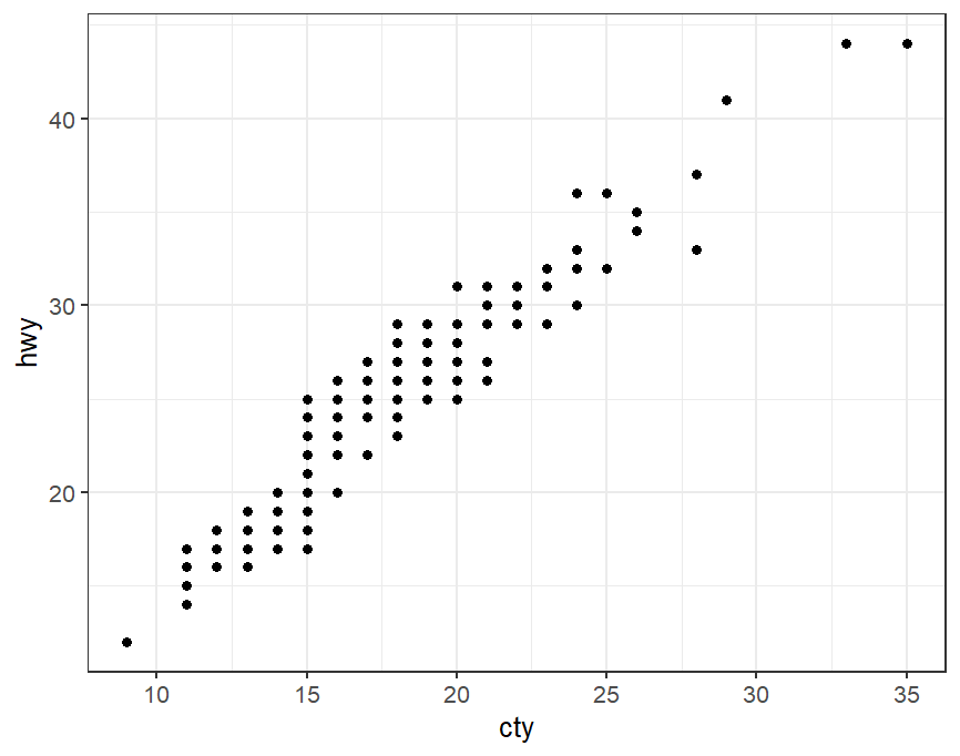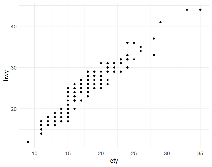
`theme_minimal()`	无边框、浅细网格
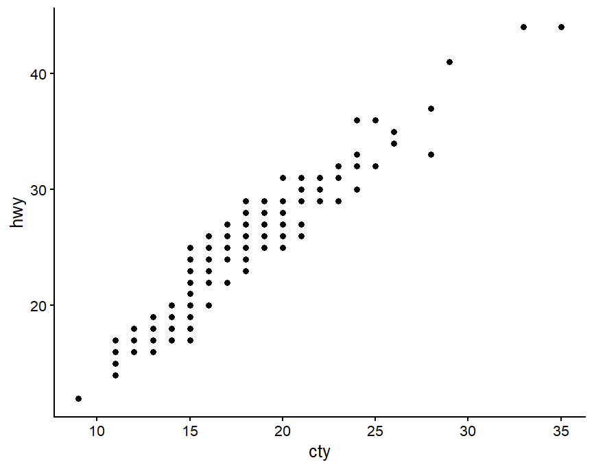
`theme_classic()`	无网格，仅保留 XY 黑色轴线
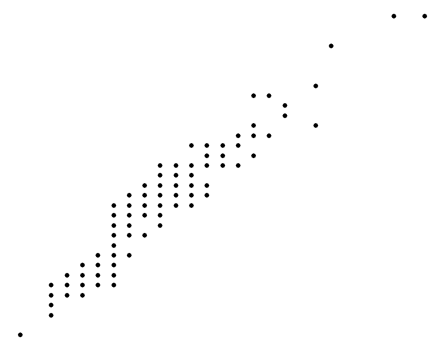
`theme_void()`	完全空白，无坐标轴、无背景

2）labs ()：

 1
 2
 3
 4
 5
 6
 7
 8
 9
10


labs(
  title = "主标题",
  subtitle = "副标题",
  caption = "图注",
  x = "X轴名称",
  y = "Y轴名称",
  color = "颜色图例标题",
  size = "大小图例标题",
  fill = "填充图例标题"
)

3）guides()：精细化控制图例

1
2
3
4
5
6
7


guides(
  映射名1 = guide_legend(参数...), # 用于普通离散 / 连续图例
  映射名2 = guide_colorbar(参数...) # 用于连续渐变色条图例
)
# override.aes：强制修改图例里图标的样式
# 图例里的圆点统一放大到size=5，不改变原图散点尺寸
# guides(color = guide_legend(override.aes = list(size = 5, alpha = 1)))

4）theme()：控制坐标轴文字、标题、网格、图例位置、边框、留白、背景等

标题相关——plot.title; plot.subtitle; plot.caption; strip.text（分面 facet_wrap 的子图标题）；

坐标轴相关——axis.title.x / axis.title.y; axis.text.x / axis.text.y; axis.line

各种绘图

散点图

最简单的绘制散点图：

1
2
3


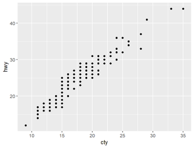
p<-ggplot(mpg,aes(x=cty,y=hwy))+
geom_point()
p

将年份映射到颜色属性：

1
2
3


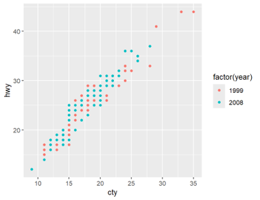
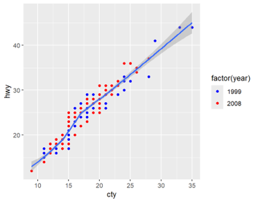
p<-ggplot(mpg,aes(x=cty,y=hwy,colour=factor(year)))+
geom_point()
p

更改点的形状属性

1
2
3


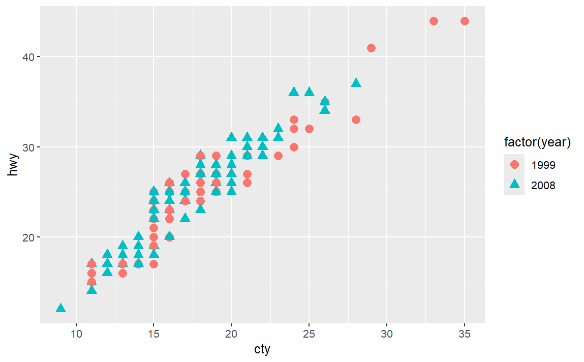
p<-ggplot(mpg,aes(x=cty,y=hwy,colour=factor(year),shape=factor(year)))+
geom_point(size=3)
p

增添平滑曲线：

 1
 2
 3
 4
 5
 6
 7
 8
 9
10
11


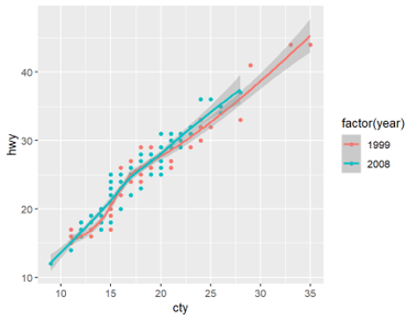
# 分开的散点按年份分两种颜色，分别拟合两条独立的拟合曲线
p<-ggplot(mpg,aes(x=cty,y=hwy,colour=factor(year)))+
geom_point()+
stat_smooth()
p

# 不分组地对全部数据拟合出一条统一的平滑曲线
p<-ggplot(mpg,aes(x=cty,y=hwy))+
geom_point(aes(colour=factor(year)))+
stat_smooth()
p

标度修改颜色取值：

1
2
3
4
5


p<-ggplot(mpg,aes(x=cty,y=hwy))+
geom_point(aes(colour=factor(year)))+
stat_smooth()+
scale_color_manual(values =c('blue','red'))
p

将排量(displ)映射到散点大小：

 1
 2
 3
 4
 5
 6
 7
 8
 9
10
11
12
13
14
15


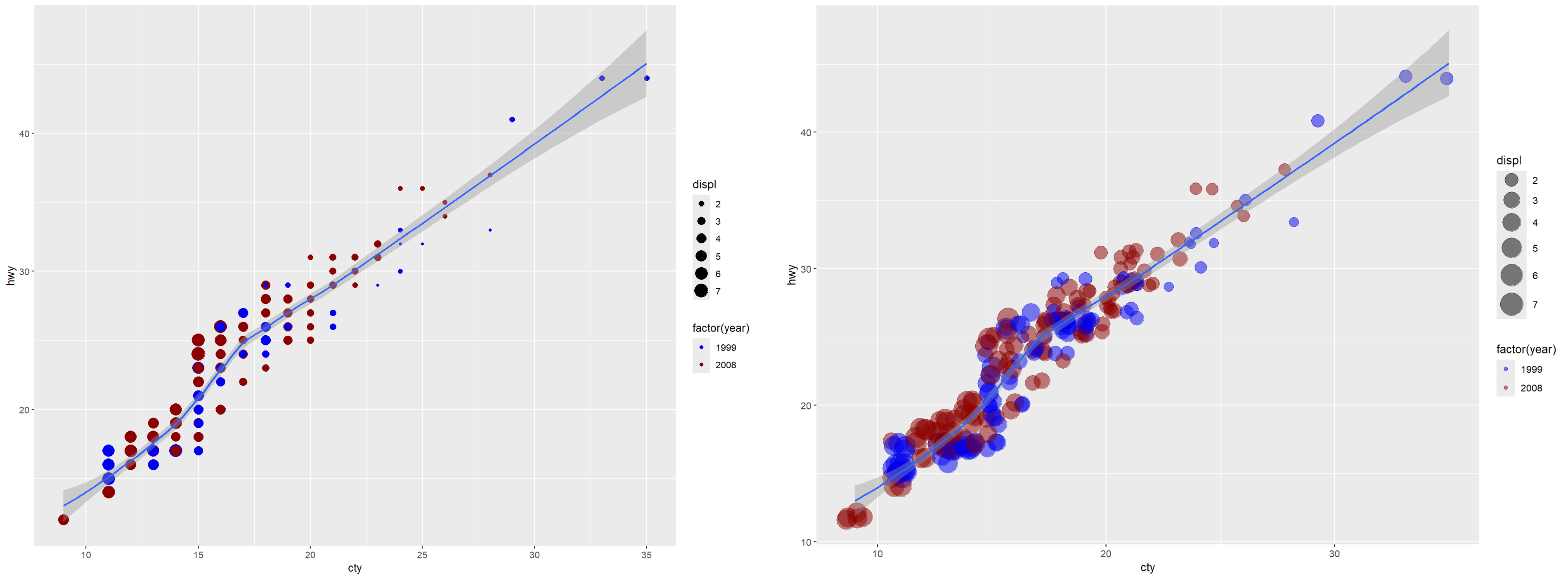
# 基础将displ数据作为点的大小标准
p<-ggplot(mpg,aes(x=cty,y=hwy))+
geom_point(aes(colour=factor(year),size=displ))+
stat_smooth()+
scale_color_manual(values=c('blue2','red4'))
p

# 调整点的大小范围、抖动和透明度;alpha=0.5调整透明度
p<-ggplot(mpg,aes(x=cty,y=hwy))+
geom_point(aes(colour=factor(year),size=displ),alpha=0.5,position="jitter")+
stat_smooth()+
scale_color_manual(values=c('blue2','red4'))+
scale_size_continuous(range=c(4,10)) 
#控制连续变量displ对应的点尺寸范围，最大为10，最小为4
p

坐标控制图形显示的范围：

1
2
3
4
5
6
7
8


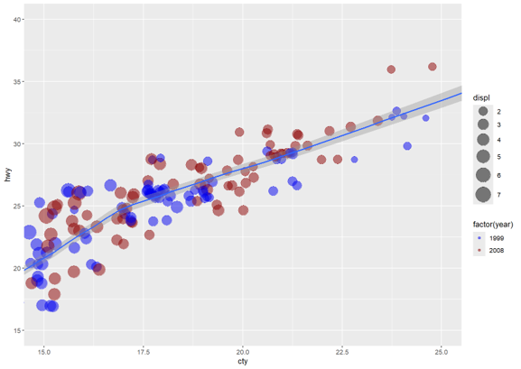
# 使用xlim和ylim限定坐标轴的范围
p<-ggplot(mpg,aes(x=cty,y=hwy))+
geom_point(aes(color=factor(year),size=displ),alpha=0.5,position="jitter")+
stat_smooth()+
scale_color_manual(values=c('blue2','red4'))+
scale_size_continuous(range=c(4,10))+
coord_cartesian(xlim=c(15,25),ylim=c(15,40))
p

利用facet分别显示不同年份的数据：

 1
 2
 3
 4
 5
 6
 7
 8
 9
10
11
12
13
14
15
16
17
18


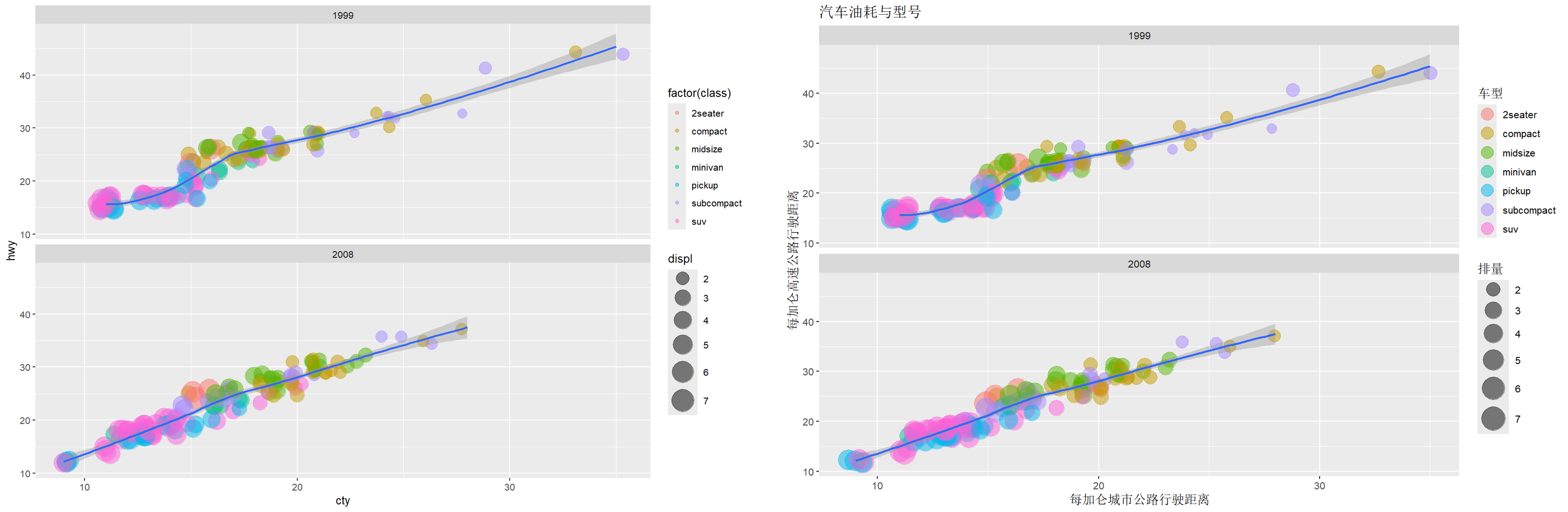
p<-ggplot(mpg,aes(x=cty,y=hwy))+
geom_point(aes(color=factor(class),size=displ),alpha=0.5,position="jitter")+
stat_smooth()+
scale_size_continuous(range=c(4,10))+
facet_wrap(~year,ncol=1) # ncol=1 上下排列两图
p

# 增添图名并精细修改图例
p<-ggplot(mpg,aes(x=cty,y=hwy))+
geom_point(aes(color=factor(class),size=displ),alpha=0.5,position="jitter")+
stat_smooth()+
scale_size_continuous(range=c(4,10))+
facet_wrap(~year,ncol=1)+
labs(title='汽车油耗与型号',y='每加仑高速公路行驶距离',x='每加仑城市公路行驶距离')+
guides(size=guide_legend(title='排量'),
    colour = guide_legend(title='车型',override.aes=list(size=5))
      )
p

直方图

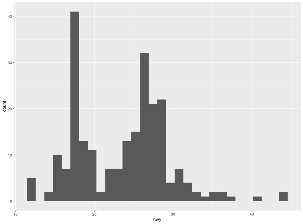
注意直方图的geom_histogram()是处理连续数值的分布，可以通过binwidth指定区间宽度；而geom_bar()是对每个数据的出现进行计数做出的柱状图。

绘制简单直方图：

1
2
3


p<-ggplot(mpg,aes(x=hwy))+
geom_histogram() # 这里由于数据mpg都是整数，geom_bar(binwidth=1)等价于geom_bar()
p

1
2
3
4


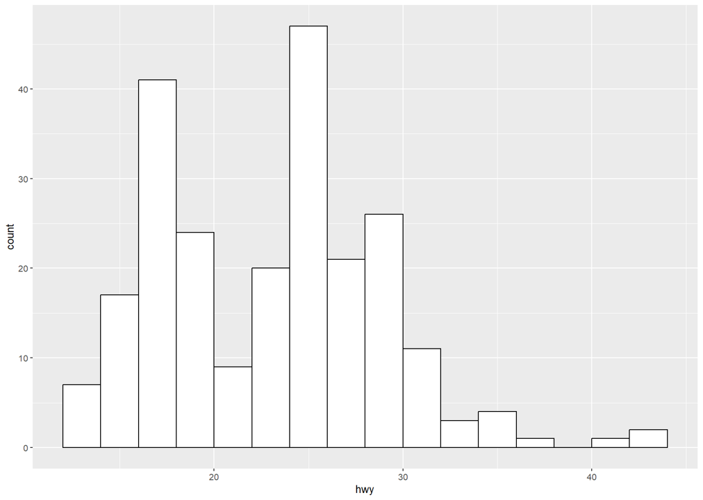
p<-ggplot(mpg,aes(x=hwy))+
geom_histogram(binwidth=2,fill='white',color='black',boundary = 30) 
p
# boundary和binwidth共同确定直方图横轴的划分。比如boundary=20，binwidth=2，那么划分线为……16，18，20，22，24，……可见不同的划分线会影响直方图的样子。

分组直方图：

 1
 2
 3
 4
 5
 6
 7
 8
 9
10


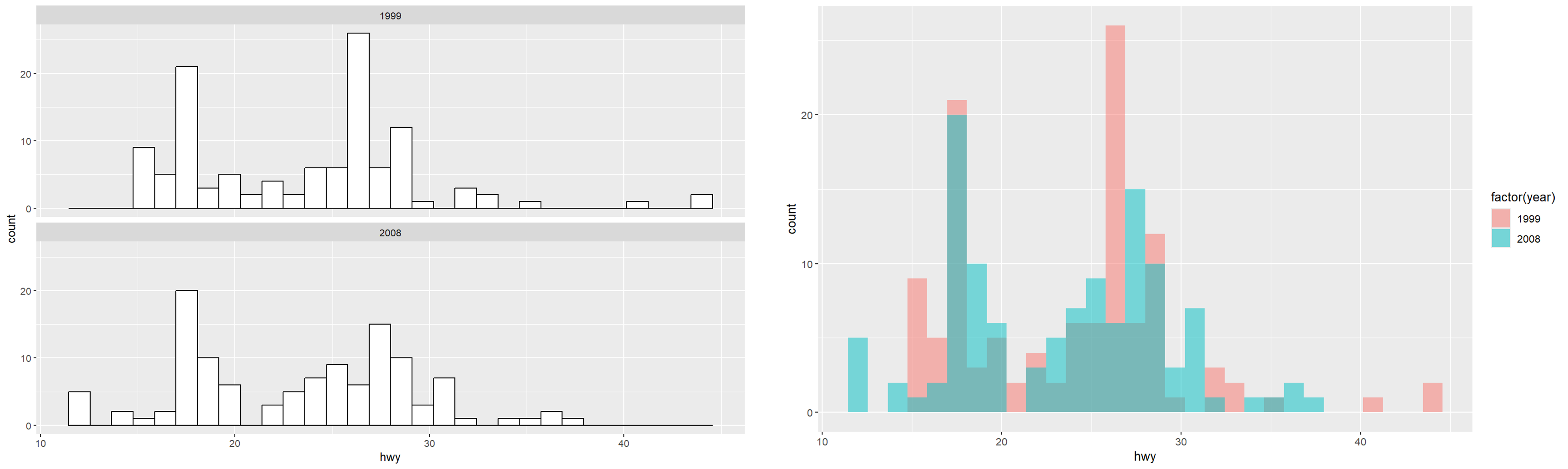
# 依据year分为2组
p<-ggplot(mpg,aes(x=hwy))+
geom_histogram(fill='white',color='black')+
facet_wrap(~year,ncol=1)
p

# 一张图中不同颜色表示分组
p<-ggplot(mpg,aes(x=hwy,fill=factor(year)))+
geom_histogram(position='identity',alpha=0.5)
p

添加密度曲线：

 1
 2
 3
 4
 5
 6
 7
 8
 9
10
11
12
13


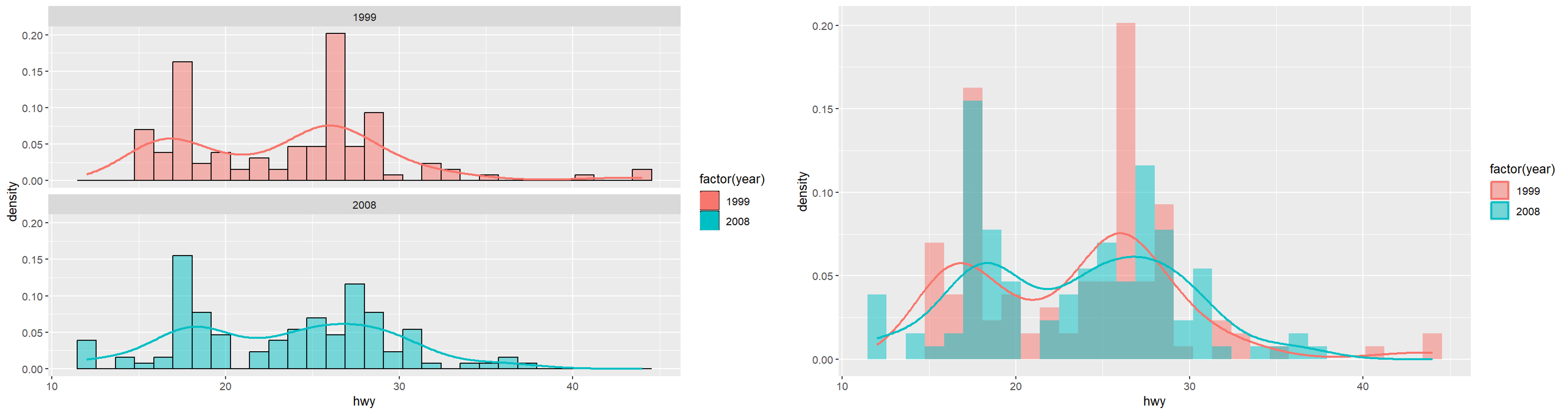
# 依据year分为2组
p<-ggplot(mpg,aes(x=hwy,y=..density..))+
geom_histogram(aes(fill=factor(year)),color='black',alpha=0.5)+
facet_wrap(~year,ncol=1)+
geom_density(aes(color=factor(year)),size=1,position='identity')
# +scale_fill_manual(values =c('blue','red')) #更改颜色可添加
p

# 一张图中不同颜色表示分组
p<-ggplot(mpg,aes(x=hwy,y=..density..,fill=factor(year)))+
geom_histogram(position='identity',alpha=0.5)+
geom_density(aes(color=factor(year)),size=1,position='identity',alpha=0)
p

柱状图

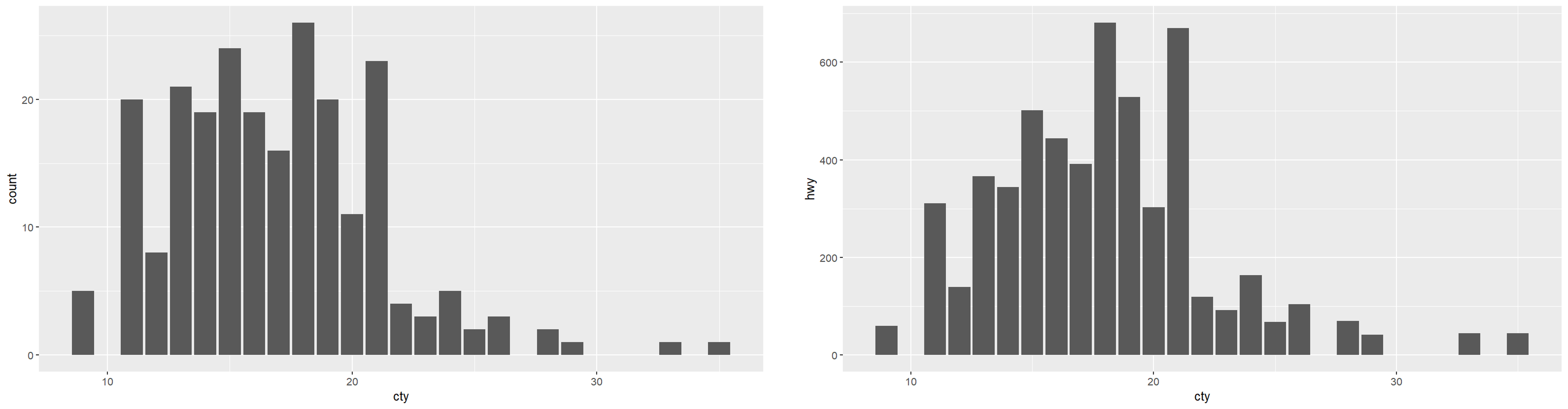
geom_bar()只有 X 分类，无现成 Y 数值，自动统计每组样本数量；而geom_col()X 是分类、Y 是你数据里已经存在的数值列，直接按给定高度画柱子。

简单柱状绘图：

1
2
3
4
5
6
7
8
9


# geom_bar()统计数量
p<-ggplot(mpg,aes(x=cty))+
geom_bar()
p

# geom_col()绘图
p<-ggplot(mpg,aes(x=cty,y=hwy))+
geom_col()
p

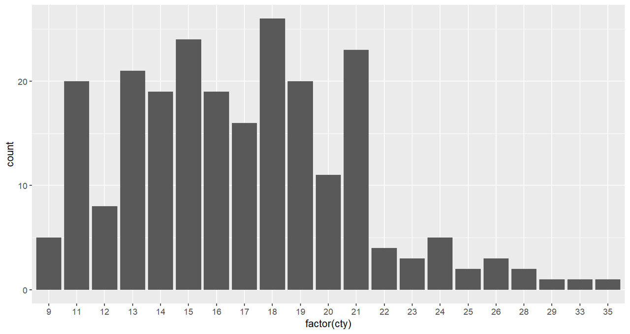
ps. 当对横轴转换成因子后，会把横轴变成连接在一起：

1
2
3


p<-ggplot(mpg,aes(x=factor(cty)))+
geom_bar()
p

绘制不同因子下柱状图：

1
2
3
4
5
6
7
8
9


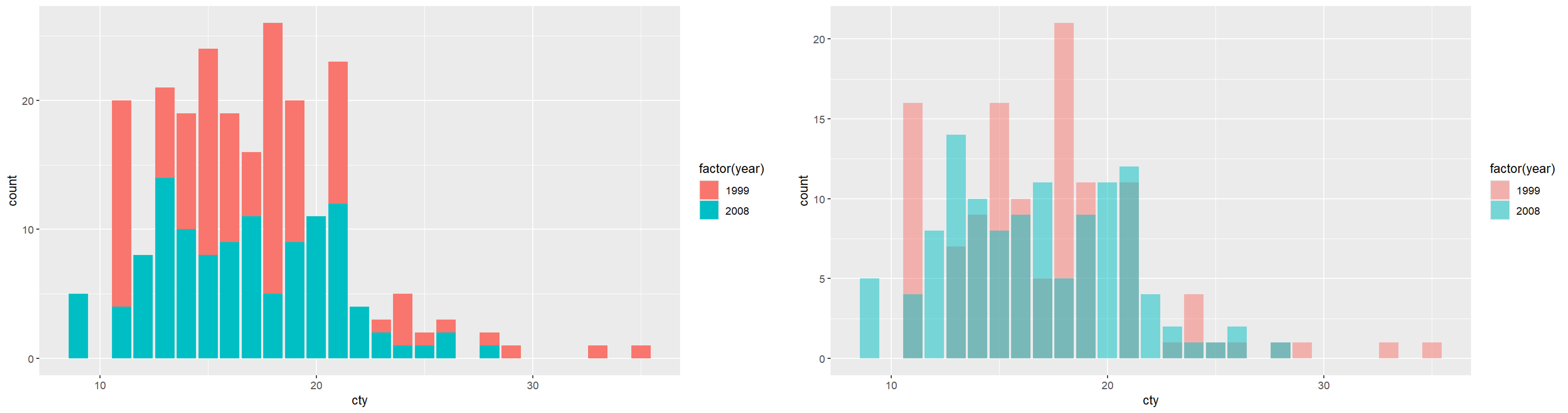
# 分开显示
p<-ggplot(mpg,aes(x=cty))+
geom_bar(aes(fill=factor(year)))
p

# 重叠显示
p<-ggplot(mpg,aes(x=cty))+
geom_bar(aes(fill=factor(year)),position='identity',alpha=0.5)
p

并立式与相对比例式：

1
2
3
4
5
6
7
8
9


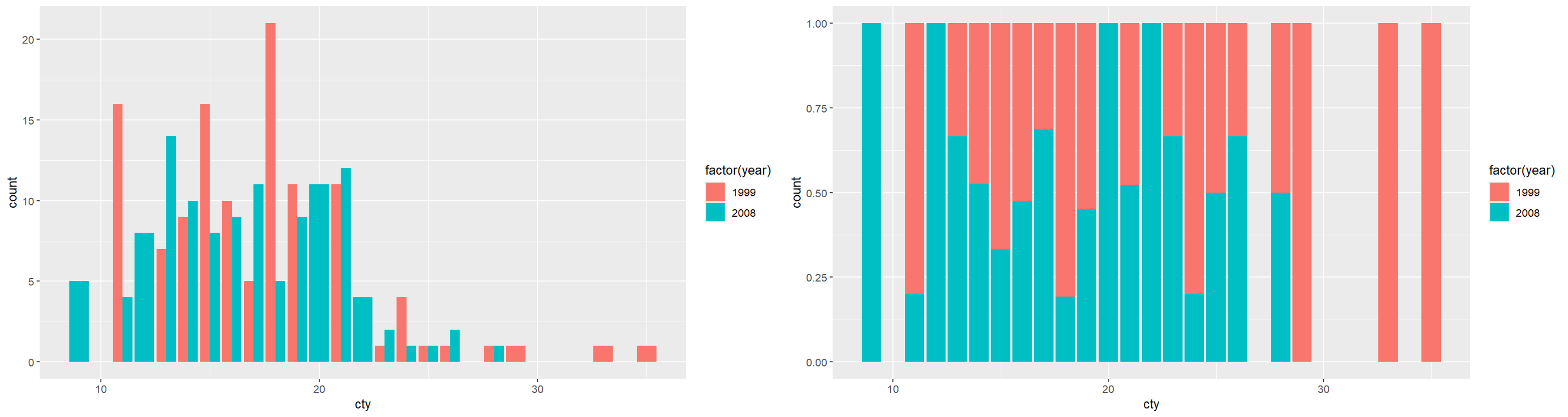
# 并立式
p<-ggplot(mpg,aes(x=cty))+
geom_bar(aes(fill=factor(year)),position='dodge')
p

# 相对比例式
p<-ggplot(mpg,aes(x=cty))+
geom_bar(aes(fill=factor(year)),position='fill')
p

克利夫兰点阵图：

用单个圆点代表每个分类的数值，默认横向排布、分类纵向排序，用来替代柱状图做多分类数值对比。

 1
 2
 3
 4
 5
 6
 7
 8
 9
10
11
12
13
14
15
16
17
18
19
20


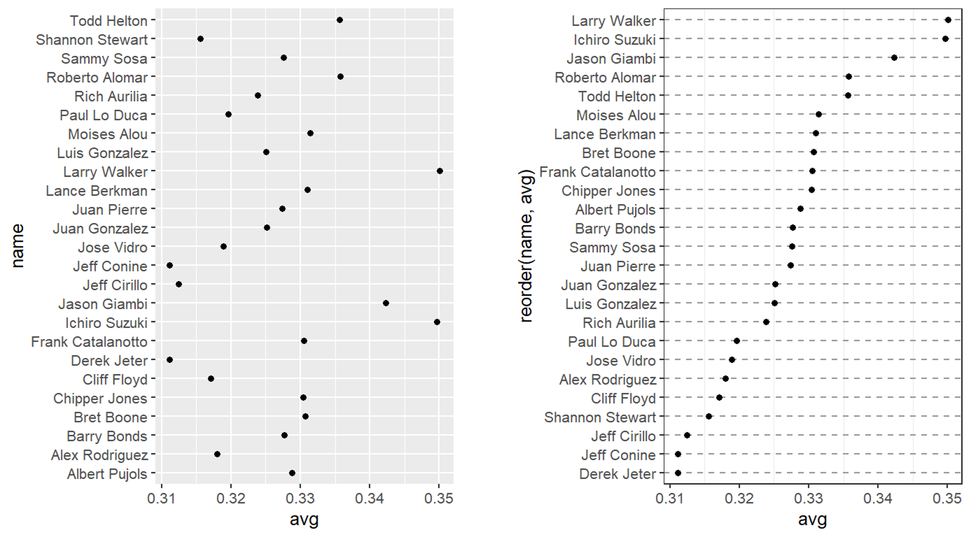
library(gcookbook) # 加载gcookbook数据集包，内置各类绘图示例数据
tophit <- tophitters2001[1:25, ] # 提取数据集前25行，取打击数据前25名球员

# 绘图主体
p<-ggplot(tophit, aes(x = avg, y = name))+
geom_point()
p

# 按照数值使用reorder()进行排序：reorder(y分类, x数值)
# 对绘图进行精修
p<-ggplot(tophit, aes(x = avg, y = reorder(name,avg)))+
geom_point()+
theme_bw()+
theme(
    panel.grid.major.x = element_blank(),
    panel.grid.minor.x = element_blank(),
    panel.grid.major.y = element_line(colour = "grey60", linetype = "dashed")
  )
# panel.grid代表绘图区域内部的网格线，分为major主网格、minor次网格
p

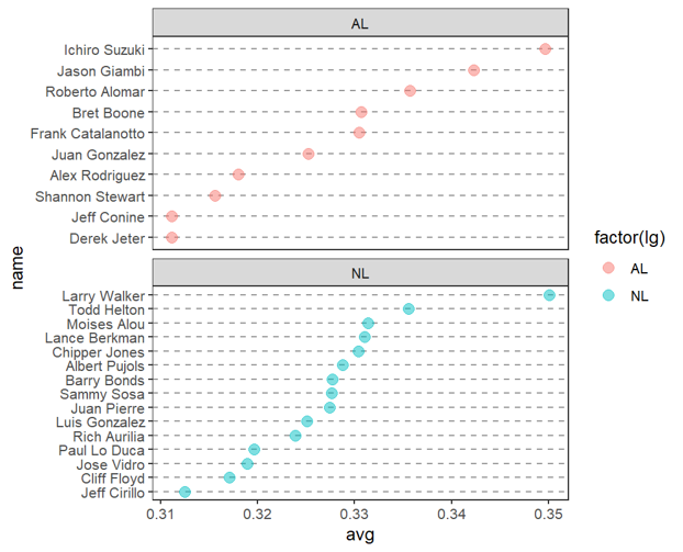
按照 lg 分组绘制克利夫兰点阵图

 1
 2
 3
 4
 5
 6
 7
 8
 9
10
11
12
13
14


# 先正确排序name
tophit$name <- reorder(tophit$name, tophit$avg)

p<-ggplot(tophit, aes(x = avg, y = name))+
geom_point(aes(color=factor(lg)), alpha = 0.5, size = 3)+
theme_bw()+
theme(
    panel.grid.major.x = element_blank(),
    panel.grid.minor.x = element_blank(),
    panel.grid.major.y = element_line(colour = "grey60", linetype = "dashed")
  )+
facet_wrap(~lg, ncol=1, scales = "free_y")
# scales="free_y"开启y轴自由，删掉空行
p

折线图

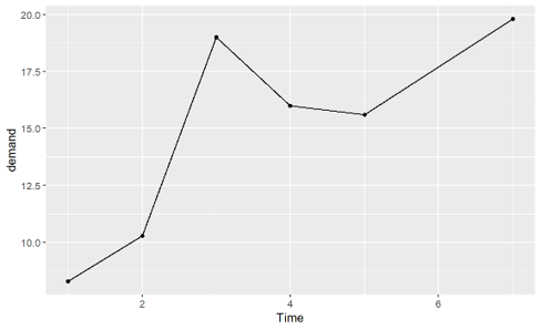
选取内置数据集BOD

简单折线图

 1
 2
 3
 4
 5
 6
 7
 8
 9
10


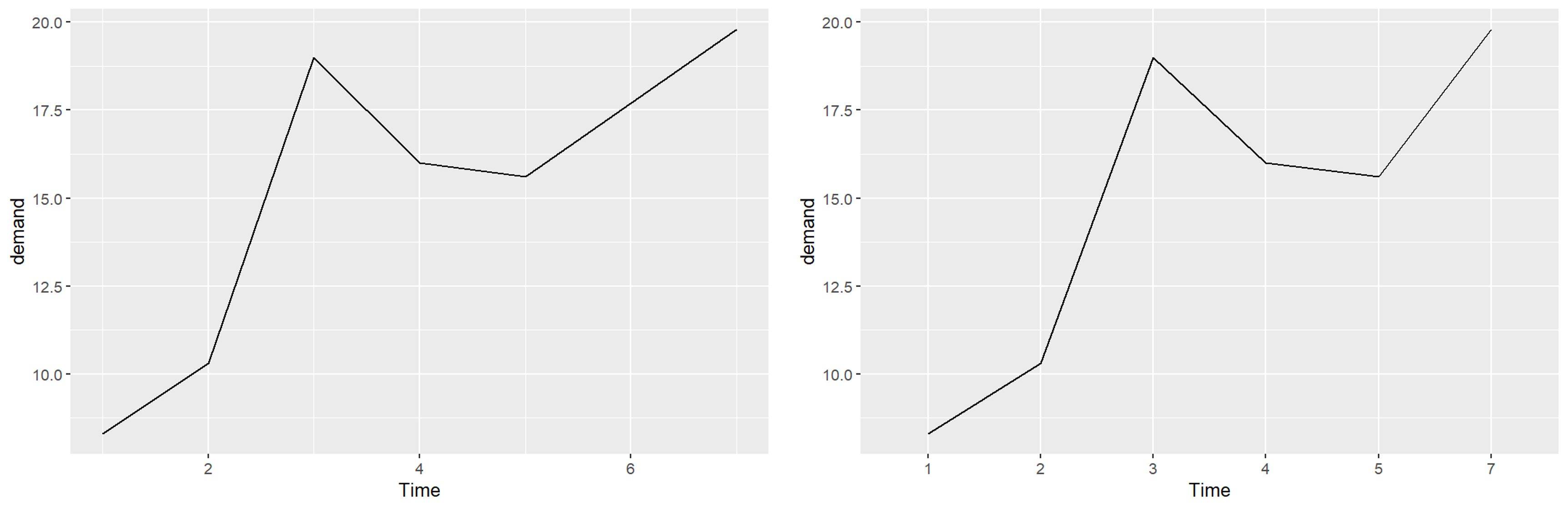
ggplot(BOD, aes(x = Time, y = demand))+
geom_line()

# 设置成因子
BOD1 <- BOD
BOD1$Time <- factor(BOD1$Time)
ggplot(BOD1, aes(x = Time, y = demand, group = 1)) +
geom_line()
# 把 Time 理解成 4 个完全互不相关的类别，每个类别下面只有 1 个样本，group = 1 把全部这些点归为同一组
# 这样绘图横轴无论数值大小是等间距的，每个类别等宽均分

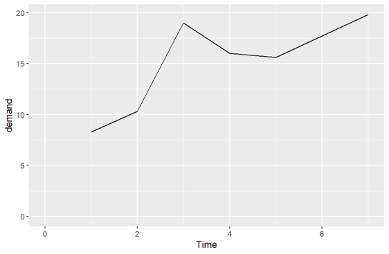
手动设置坐标轴的范围：

1
2
3
4


p <- ggplot(BOD, aes(x = Time, y = demand))+
geom_line()+
coord_cartesian(xlim = c(0, max(BOD$Time)), ylim = c(0, max(BOD$demand)))
p

带点折线图

1
2
3
4


p <- ggplot(BOD, aes(x = Time, y = demand)) +
geom_line() +
geom_point()
p

多条折线图

1
2
3
4
5
6
7
8
9


library(gcookbook)
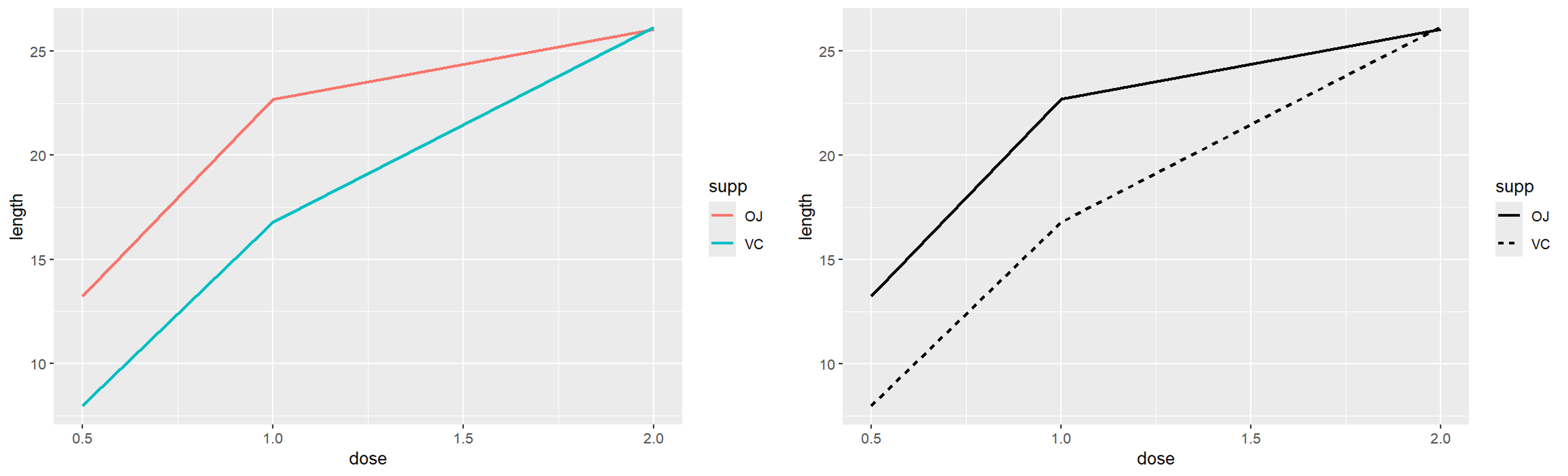
# 分别使用线条颜色和样式区分两组
p <- ggplot(tg, aes(x = dose, y = length, color = supp))+
geom_line(linewidth = 1)
p

p <- ggplot(tg, aes(x = dose, y = length, linetype = supp))+
geom_line(linewidth = 1)
p

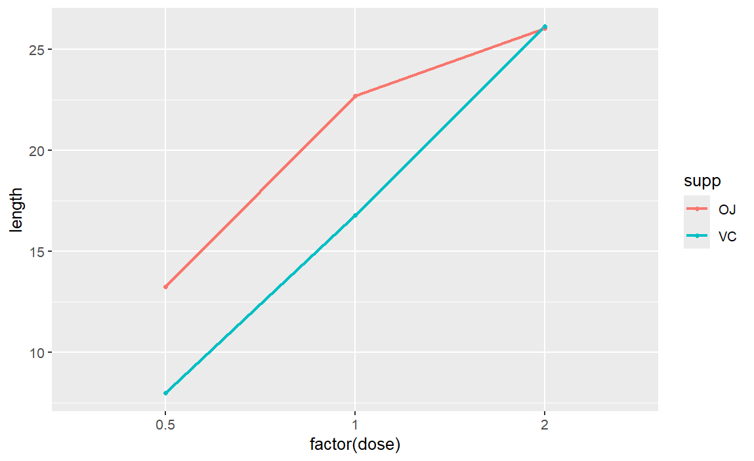
当 x 变量是因子时，把这些当成类别来看待，而不是连续的数值

1
2
3
4


p <- ggplot(tg, aes(x = factor(dose), y = length, color = supp, group = supp))+
geom_line(linewidth = 1)+
geom_point(size = 1)
p

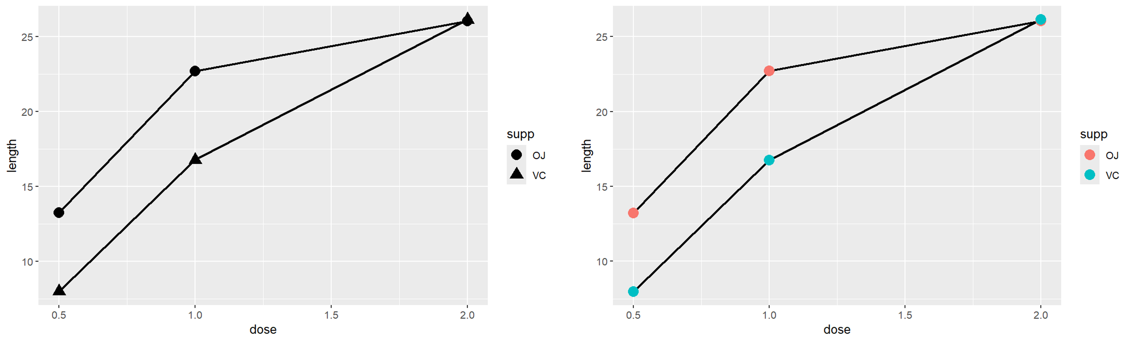
一定要正确分组，否则容易出现一个 x 对应多个 y 值的情况，采取shape、color、fill、linetype等达到目的

1
2
3
4
5
6
7
8
9


p <- ggplot(tg, aes(x = dose, y = length, shape = supp))+
geom_line(linewidth = 1)+
geom_point(size = 4)
p

p <- ggplot(tg, aes(x = dose, y = length, fill = supp))+
geom_line(linewidth = 1)+
geom_point(size = 4, aes(color = supp))
p

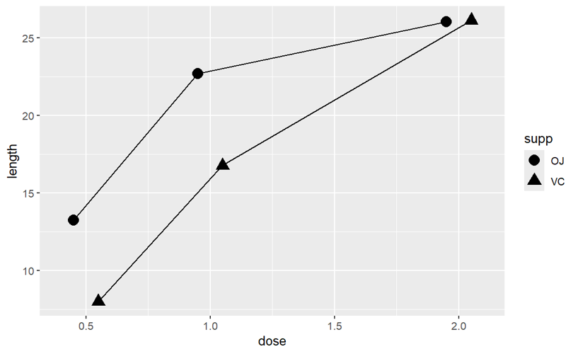
当发现存在点与点之间的重叠时，想避免重叠可以在geom_point()和geom_line中增添position指令

1
2
3
4


p <- ggplot(tg, aes(x = dose, y = length, shape = supp)) +
geom_line(position = position_dodge(0.2)) +         
geom_point(position = position_dodge(0.2), size = 4) 
p

外观

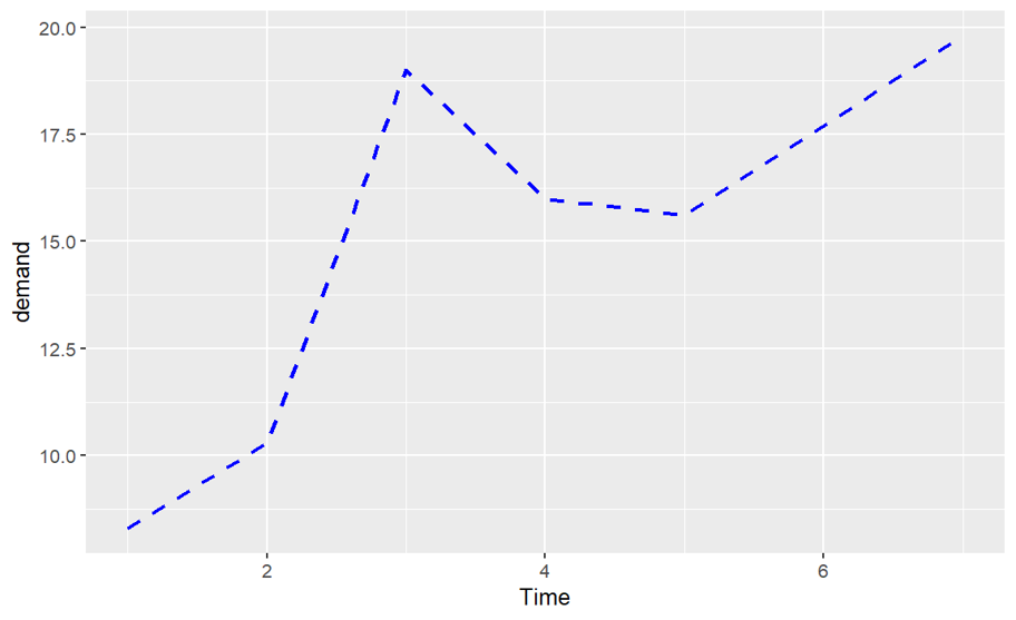
可以调整线条的参数控制来改变折线的外观，如linetype、size、colour、color

1
2
3
4


p <- ggplot(BOD, aes(x = Time, y = demand)) +
geom_line(linetype = "dashed", size = 1, colour = "blue")
p
# 绘制虚线

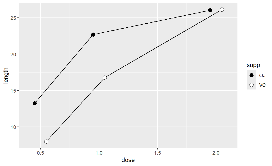
改变点的外观

1
2
3
4
5
6
7


library(gcookbook)
pd <- position_dodge(0.2)
p <- ggplot(tg, aes(x = dose, y = length, fill = supp)) +
geom_line(position = pd) +
geom_point(shape = 21, size = 3, position = pd) +
scale_fill_manual(values = c("black","white"))
p

带阴影图表

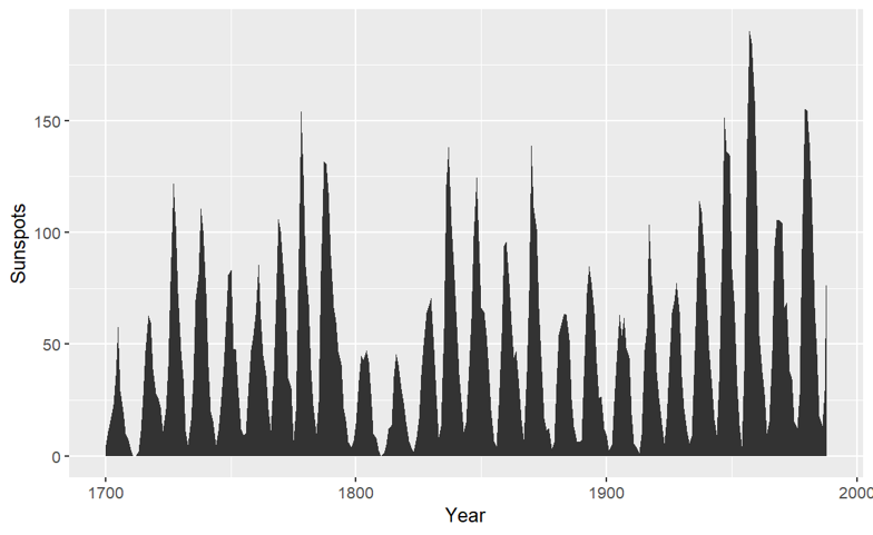
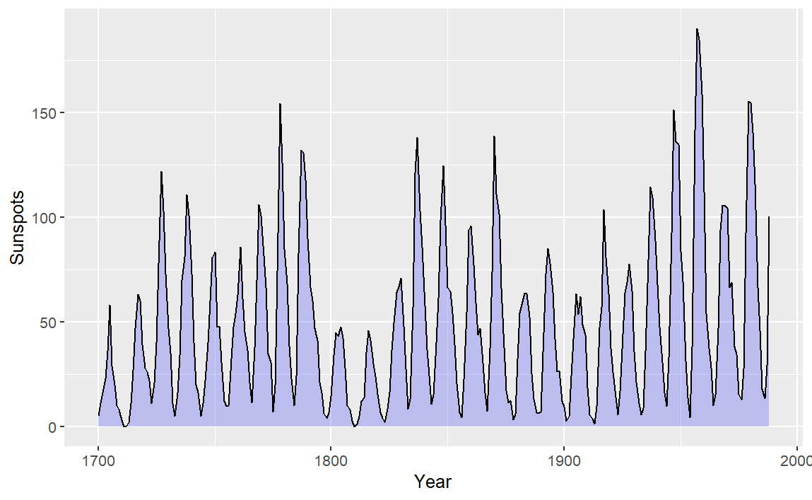
使用geom_area()可以获得阴影区域

1
2
3
4
5
6
7
8


# 把 sunsport.year 时间序列转换成数据框类型
sunspotyear <- data.frame(
Year = as.numeric(time(sunspot.year)),
Sunspots = as.numeric(sunspot.year))

p <- ggplot(sunspotyear, aes(x = Year, y = Sunspots)) +
geom_area()
p

美化阴影图表，改变轮廓和颜色

1
2
3
4


p <- ggplot(sunspotyear, aes(x = Year, y = Sunspots)) +
geom_area(color = "black", fill = "blue", alpha = 0.2)+
geom_line()
p

堆叠面积图

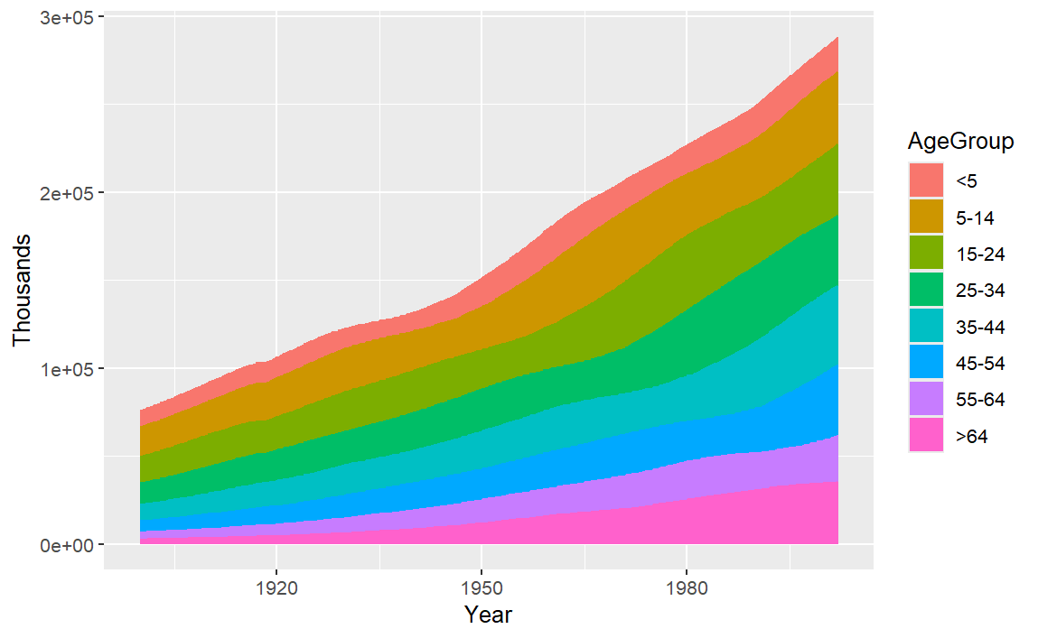
多条面积图，一层层往上摞在一起，每个分组都是从上一组的顶部开始往上画

1
2
3
4


library(gcookbook)
p <- ggplot(uspopage, aes(x = Year, y = Thousands, fill = AgeGroup))+
geom_area()
p

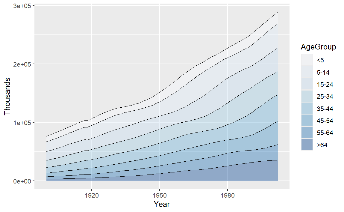
更改为渐变色

1
2
3
4
5
6
7


p <- ggplot(uspopage, aes(x = Year, y = Thousands, fill = AgeGroup, order = dplyr::desc(AgeGroup)))+
geom_area(colour = NA, alpha = .4)+
scale_fill_brewer(palette = "Blues")+
geom_line(position = "stack", linewidth = .2)
p
# 使用 RColorBrewer 配色方案，全部使用蓝色系的不同深浅给各个 AgeGroup 分组上色，由于是修改 fill 映射的配色，所以 中间是 fill 而不是 scale_color_brewer
# position = "stack"不同于position = "identity"，前者是 y 位置堆叠的画线，而后者是实际 y 数值的画线

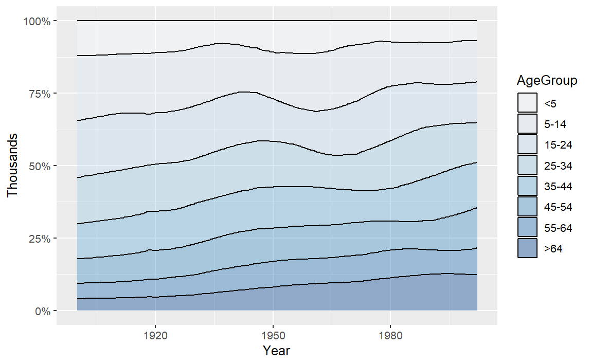
将上述的堆叠面积图再绘制成有一定比例的堆叠面积图

1
2
3
4
5


p <- ggplot(uspopage, aes(x = Year, y = Thousands, fill = AgeGroup, order = dplyr::desc(AgeGroup)))+
geom_area(position = "fill", colour = "black", alpha = .4)+
scale_fill_brewer(palette = "Blues")+
scale_y_continuous(labels = scales::percent)
p

添加置信区间

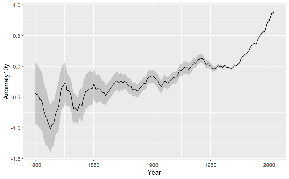
选取 climate 数据集中 1800 年至 2004 年平均温度和 95% 置信区间。

 1
 2
 3
 4
 5
 6
 7
 8
 9
10
11


# 数据预处理
library(gcookbook)
library(tidyverse)
climate_mod <- climate %>%
filter(Source == "Berkeley") %>%
select(Year, Anomaly10y, Unc10y)

p <- ggplot(climate_mod, aes(x = Year, y = Anomaly10y))+
geom_ribbon(aes(ymin = Anomaly10y - Unc10y, ymax = Anomaly10y + Unc10y), alpha = .2)+
geom_line()
p

拟合回归

要向散点图添加线性回归线，需要添加不同组件：stat_smooth()、method = lm lm() sp

如下为普通绘图：

1
2
3
4
5
6
7
8
9


library(gcookbook)
p <- ggplot(heightweight, aes(x = ageYear, y = heightIn))+
geom_point() +
stat_smooth(method = lm)
p
# 注意一定要加 method = lm 表示普通线性回归，否则默认为method = "loess" 局部加权非线性平滑
# 默认是 level = 0.95 95%置信区间
# stat_smooth(method = lm, level = 0.99) 99%置信区间
# stat_smooth(method = lm, se = FALSE) 无置信区间

更改点和线的颜色

1
2
3
4


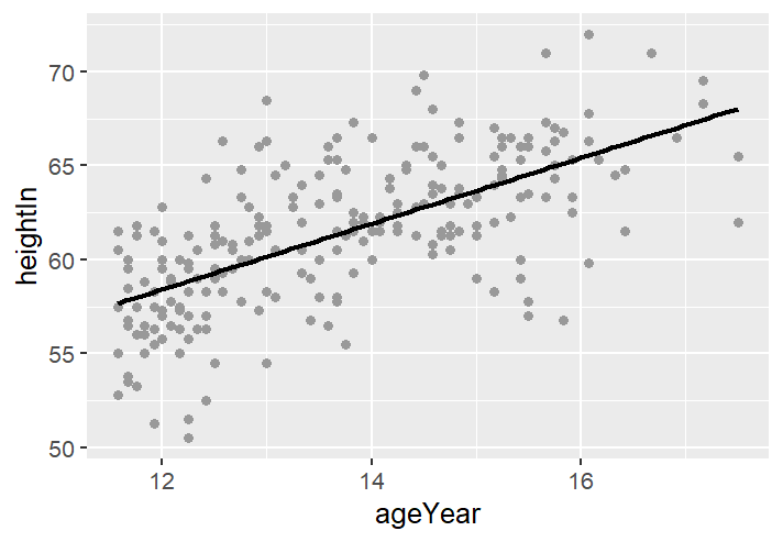
p <- ggplot(heightweight, aes(x = ageYear, y = heightIn))+
geom_point(color = "grey60") +
stat_smooth(method = lm, se = FALSE, color = "black")
p

允许模型外推

 1
 2
 3
 4
 5
 6
 7
 8
 9
10
11


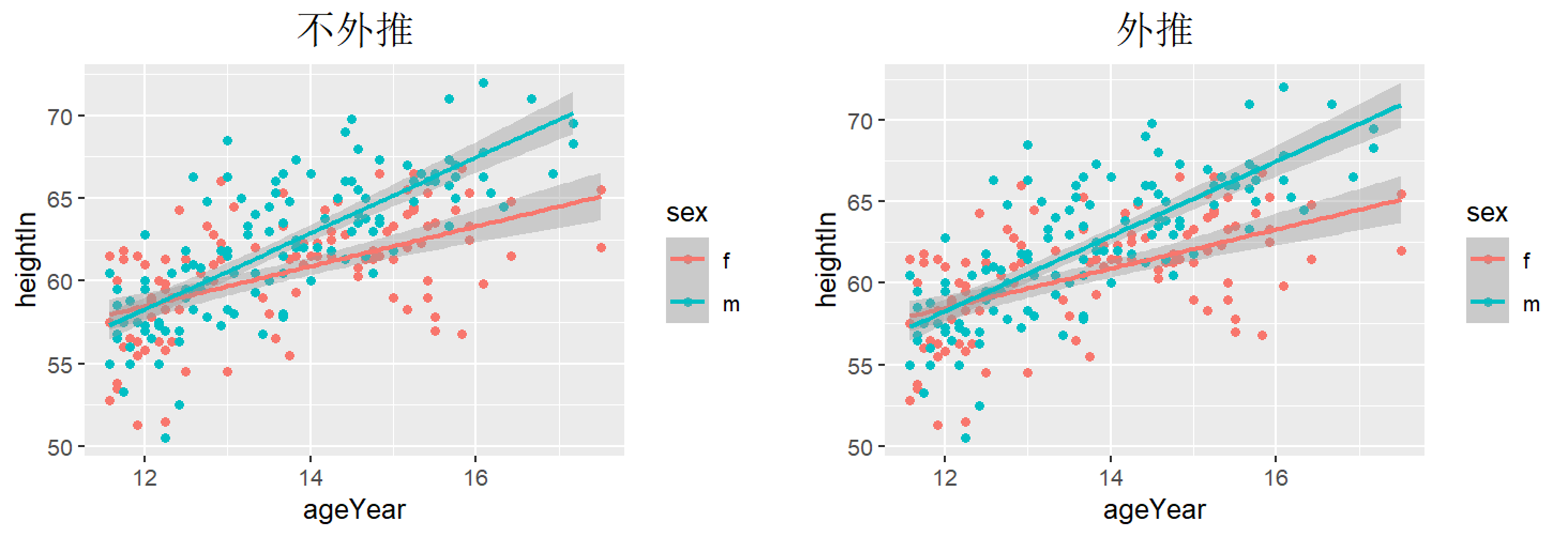
p <- ggplot(heightweight, aes(x = ageYear, y = heightIn, color = sex))+
geom_point()+
geom_smooth(method = lm, fullrange = TRUE)+
labs(title = "外推")+
  theme(
    plot.title = element_text(
      size = 16,       
      hjust = 0.5,      
      vjust = 1,        
      color = "black"))
p

添加模型系数的注释

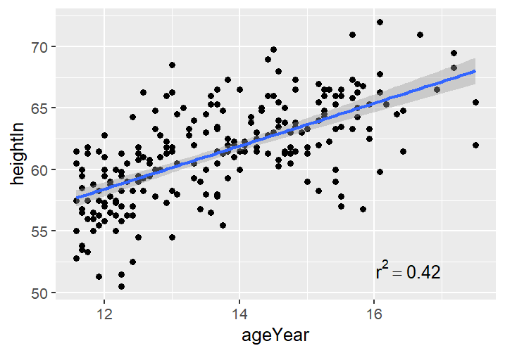
要为图中添加简单文本，只需添加注释即可。可以通过线性拟合明确拟合的解释度 $R^2$ ，再添加到拟合图中

 1
 2
 3
 4
 5
 6
 7
 8
 9
10
11


library(gcookbook)
model <- lm(heightIn ~ ageYear, heightweight)
# lm(y ~ x, data)
summary(model)

p <- ggplot(heightweight, aes(x = ageYear, y = heightIn))+
geom_point()+
geom_smooth(method = lm)+
annotate("text", x = 16.5, y = 52, label = "r^2 == 0.42", parse = TRUE)
p
# parse = TRUE 告诉 R label里面是的数学表达式而非文本

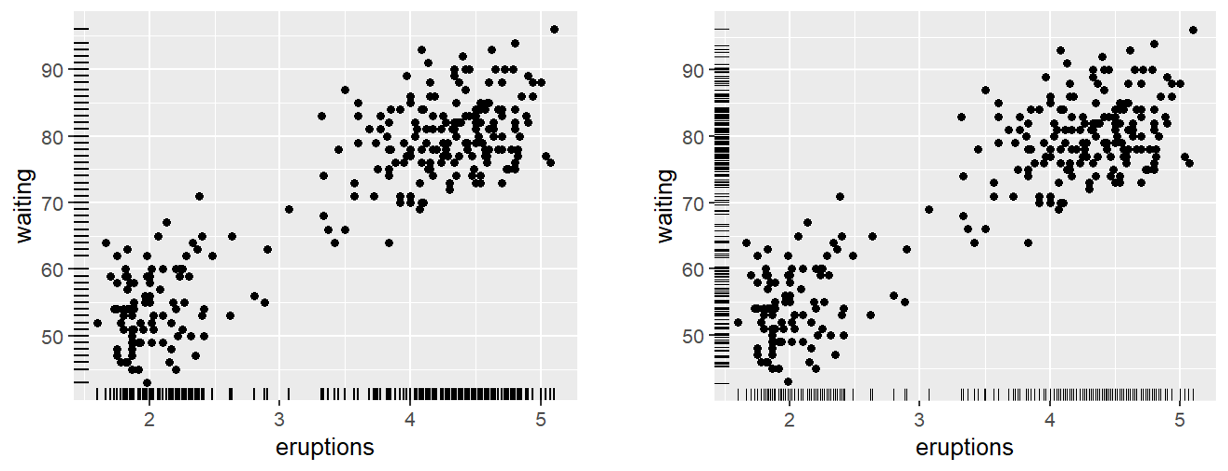
边缘地毯图

边缘地毯图本质上是一种一维散点图，可用于可视化数据在每个轴上的分布。

 1
 2
 3
 4
 5
 6
 7
 8
 9
10


p <- ggplot(faithful, aes(x = eruptions, y = waiting)) +
geom_point() +
geom_rug()
p

# 指定尺寸来调整线的位置
p <- ggplot(faithful, aes(x = eruptions, y = waiting)) +
geom_point() +
geom_rug(position = "jitter", size = 0.2)
p

标记点

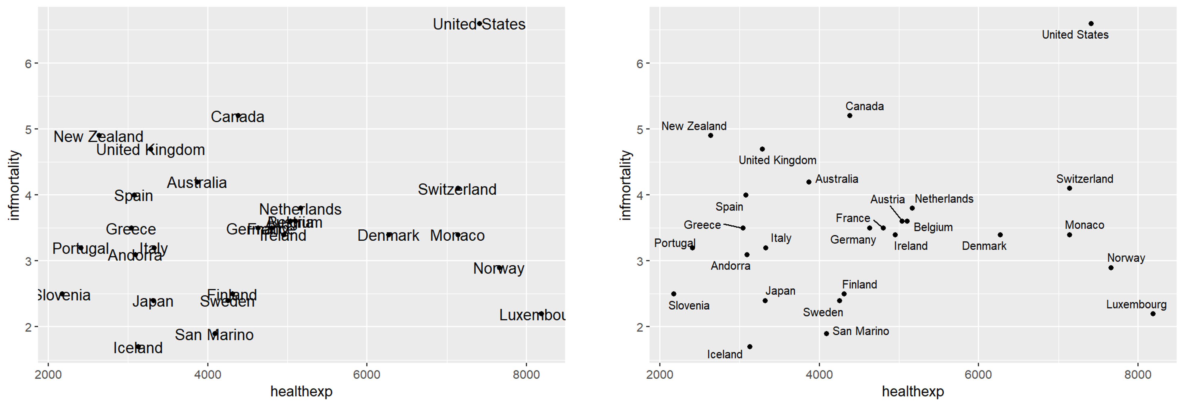
想要给散点图中的点添加标签，使用 annotate 时要指定坐标和标签，需要反复调整，因此使用 geom_text 。

 1
 2
 3
 4
 5
 6
 7
 8
 9
10
11
12
13
14
15
16


# 先筛选数据
countries_sub <- countries %>%
filter(Year == 2009 & healthexp > 2000)

# 重叠情况明显
p <- ggplot(countries_sub, aes(x = healthexp, y = infmortality))+
geom_point()+
geom_text(aes(label = Name), size = 4)
p

# 使用 ggrepel 包中 geom_text_repel() 函数代替 geom_text()
library(ggrepel)
p <- ggplot(countries_sub, aes(x = healthexp, y = infmortality))+
geom_point()+
geom_text_repel(aes(label = Name), size = 3)
p

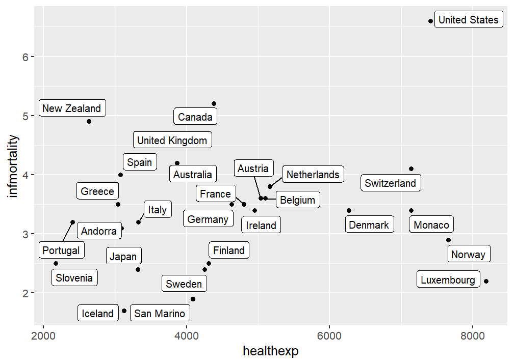
同样地还可以用 geom_label_repel() 为标签增添一个外框

1
2
3
4


p <- ggplot(countries_sub, aes(x = healthexp, y = infmortality))+
geom_point()+
geom_label_repel(aes(label = Name), size = 3)
p

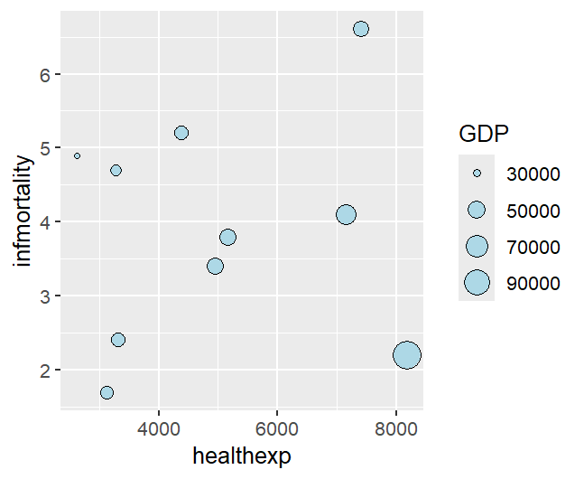
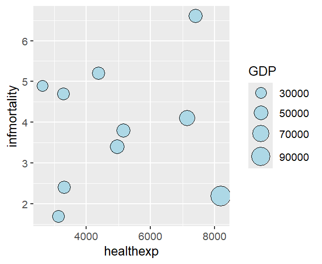
气球图

气球图由 x、y 决定点的位置，size 映射第三个数值变量

 1
 2
 3
 4
 5
 6
 7
 8
 9
10


library(gcookbook)
countrylist <- c("Canada", "Ireland", "United Kingdom", "United States", "New Zealand", "Iceland", "Japan", "Luxembourg", "Netherlands", "Switzerland")
cdat <- countries %>%
filter(Year == 2009 & Name %in% countrylist)

p <- ggplot(cdat, aes(x = healthexp, y = infmortality, size = GDP))+
geom_point(shape = 21, color = "black", fill = "lightblue")
p
# 注意这里绘制点的时候一定要有 shape = 21，因为默认点的形状是 shape = 19 实心原点；
# 而 shape = 21 是带边框的圆点

映射到面积

注意上面代码直接映射 size 是控制点的半径，要想与面积成正比需要采用 scale_size_area()

1
2
3
4


p <- ggplot(cdat, aes(x = healthexp, y = infmortality, size = GDP))+
geom_point(shape = 21, color = "black", fill = "lightblue")+
scale_size_area(max_size = 8)
p

频数气泡矩阵图

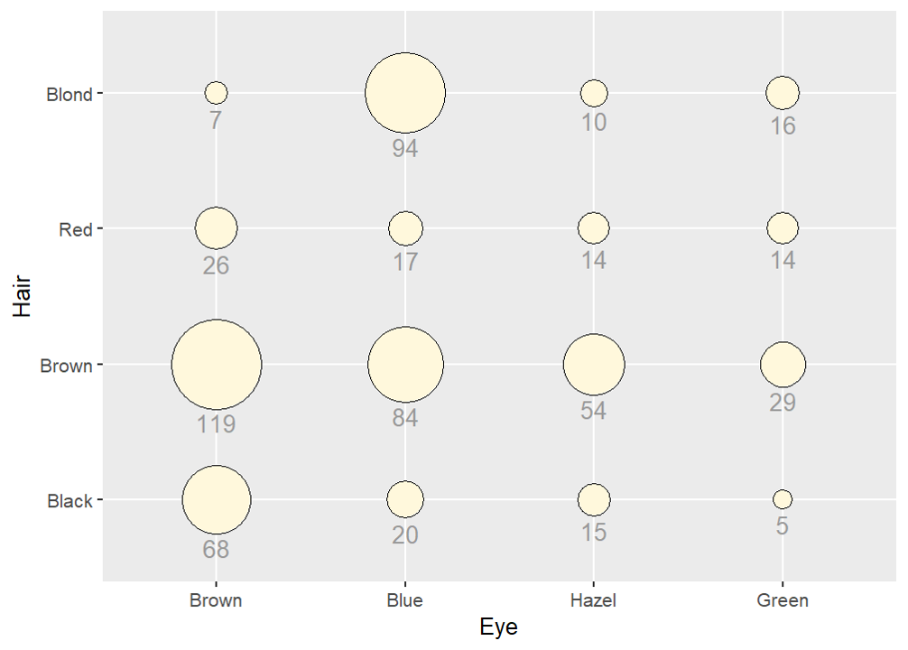
使用气球图在网格上表示数值也很有用，其中 x 轴和 y 轴为类别

 1
 2
 3
 4
 5
 6
 7
 8
 9
10
11
12
13
14
15
16
17
18
19
20
21
22


hec <- as.data.frame(HairEyeColor)
#    Hair   Eye  Sex Freq
# 1 Black Brown Male   32
# 2 Brown Brown Male   53
# 3   Red Brown Male   10 ……

# 不分性别地合并相同发色和眼色
hec_total <- hec %>%
group_by(Hair, Eye) %>%
summarise(total = sum(Freq), .groups = "drop")
# summarise() 按组压缩数据，每组输出 1 行，生成新的汇总列
# .groups="drop" 全部取消分组，返回普通无分组 tibble

p <- ggplot(hec_total, aes(x = Eye, y = Hair, size = total))+
geom_point(shape = 21, colour = "black", fill = "cornsilk")+
scale_size_area(max_size = 20, guide = FALSE)+
geom_text(
aes(y = as.numeric(as.factor(Hair)) - sqrt(total)/34, label = total), 
vjust = 1.3, 
size = 4, 
colour = "grey60")
p

气泡图

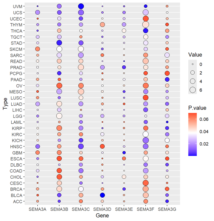
如下一个不同癌症中重点基因的表达上调和下调情况，数据集为data，行名为癌症类型，列名为基因

 1
 2
 3
 4
 5
 6
 7
 8
 9
10
11
12
13
14
15
16
17
18
19
20
21
22
23
24
25


# 数据预处理
library(tidyverse)
data$Type <- rownames(data)
data1 <- data %>%
  pivot_longer(
	cols = -Type, # 除去Type这列全部要拉长
	names_to = "Gene",
    values_to = "Value"
)
# pivot_longer() 用于宽表格 → 长表格

data1$P.value <- runif(length(rownames(data1)), 0, 0.07)
# 随机数生成P值，方便演示
# 准备好的数据框data1分为4列：Type, Gene, Value, P.value

# 绘制气泡图，渐变颜色是 P.value 大小，气泡大小是值的大小
p <- ggplot(data1, aes(x = Gene, y = Type))+
geom_point(shape = 21, aes(fill = P.value, size = Value))+
scale_size_continuous(range = c(1,6))+
scale_fill_gradient2(
    low = "blue",
    mid = "white",
    high = "red",
    midpoint = median(data1$P.value))
p

ps. 对比区分：

`scale_fill_gradient()`	单向连续渐变
`scale_fill_gradient2()`	发散渐变，有中间零点
`scale_fill_manual()`	只用于离散分类变量

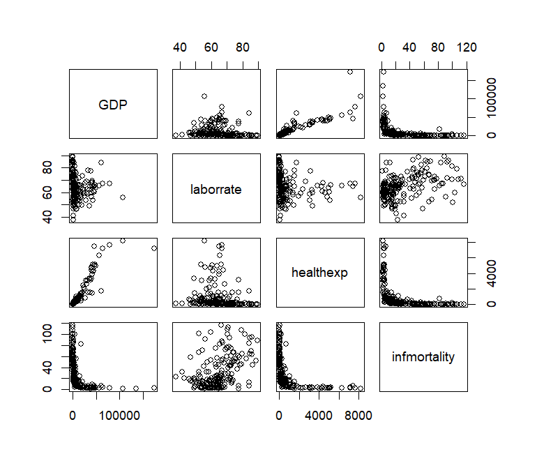
散点矩阵图

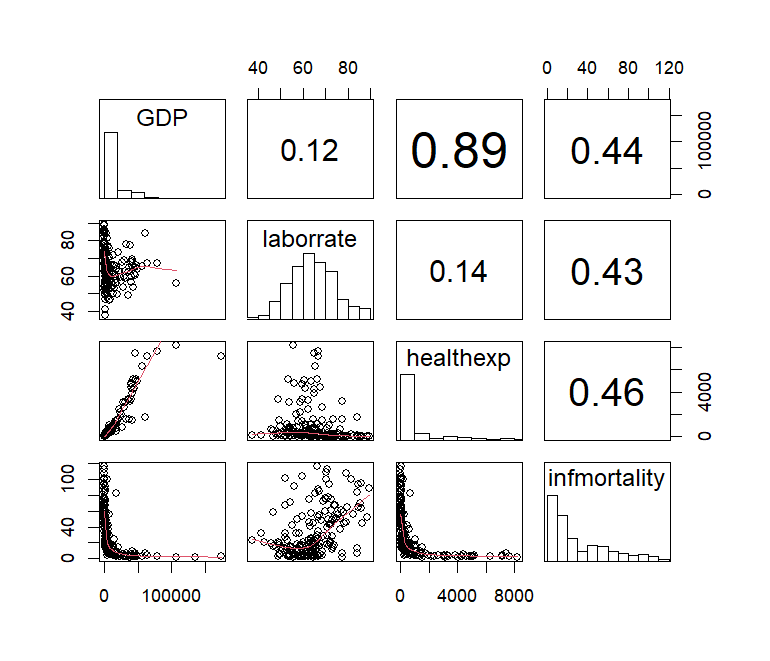
散点矩阵图是把多组数值变量，两两全部画散点图，拼成一个矩阵网格，直接使用内置的 pairs() 函数即可

1
2
3
4
5
6
7
8


library(gcookbook)
c2009 <- countries %>%
  filter(Year == 2009) %>%
  select(Name, GDP, laborrate, healthexp, infmortality)

# 使用除了 name 以外的所有变量
c2009_num <- select(c2009, -Name)
pairs(c2009_num)

使用自定义，显示每对变量的相关系数而非散点图，同时对角线显示每个变量的直方图，由此定义下列函数绘图

 1
 2
 3
 4
 5
 6
 7
 8
 9
10
11
12
13
14
15
16
17
18
19
20
21
22
23
24
25
26
27
28
29
30


panel.cor <- function(x, y, digits = 2, prefix = "", cex.cor, ...) {
  usr <- par("usr")
  on.exit(par(usr))
  par(usr = c(0, 1, 0, 1))
  r <- abs(cor(x, y, use = "complete.obs"))
  txt <- format(c(r, 0.123456789), digits = digits)[1]
  txt <- paste(prefix, txt, sep = "")
  if (missing(cex.cor)) cex.cor <- 0.8/strwidth(txt)
  text(0.5, 0.5, txt, cex =  cex.cor * (1 + r) / 2)
}

panel.hist <- function(x, ...) {
  usr <- par("usr")
  on.exit(par(usr))
  par(usr = c(usr[1:2], 0, 1.5) )
  h <- hist(x, plot = FALSE)
  breaks <- h$breaks
  nB <- length(breaks)
  y <- h$counts
  y <- y/max(y)
  rect(breaks[-nB], 0, breaks[-1], y, col = "white", ...)
}

# 绘图部分增添 loess 平滑线
pairs(
  c2009_num,
  upper.panel = panel.cor,
  diag.panel  = panel.hist,
  lower.panel = panel.smooth
)

盒状图

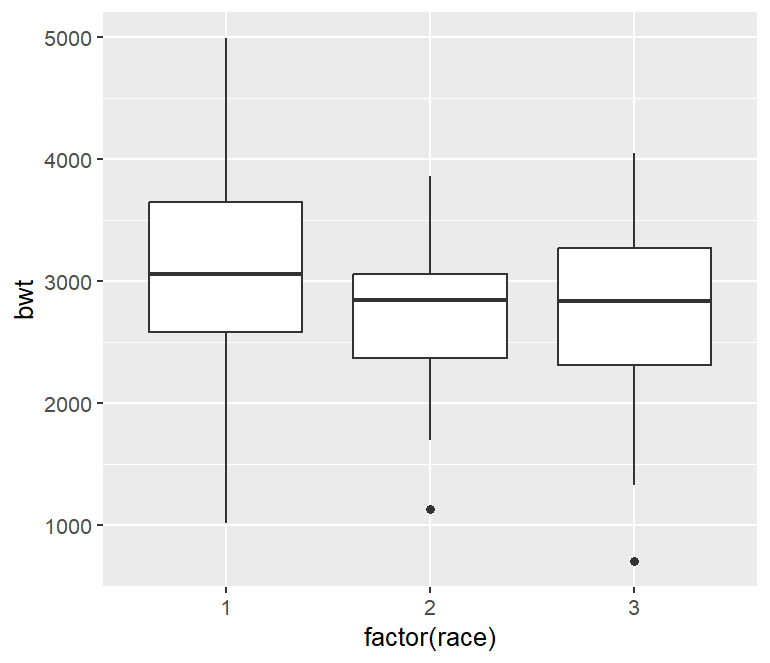
简单盒状图

1
2
3
4
5
6
7


library(MASS) 
p <- ggplot(birthwt, aes(x = factor(race), y = bwt))+
geom_boxplot()
p
# 一定要转变成 factor 类型，变成离散因子，才能分组统计画箱子
# 这里 geom_boxplot() 里面可以 width = 0.5 为例调整宽度
# 更改离群点的大小和形状：outlier.size = 1.5, outlier.shape = 21

添加刻度

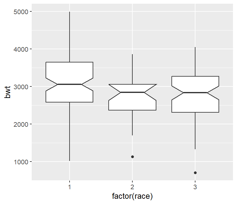
在箱线图上添加刻度可以来评估中位数是否不同

1
2
3
4


p <- ggplot(birthwt, aes(x = factor(race), y = bwt))+
geom_boxplot(notch = TRUE)
# notch = TRUE 表示画缺口箱线图，初步比较中位数差异是否显著
p

添加均值标记

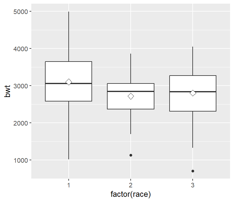
可以像箱线图中添加菱形表示平均值

1
2
3
4
5
6


p <- ggplot(birthwt, aes(x = factor(race), y = bwt))+
geom_boxplot()+
stat_summary(fun = mean, geom = "point", shape = 23, size = 3, fill = "white")
# fun = mean 表示计算每组 y 的均值
# geom = "point" 表示是用点来把几何对象画出来
p

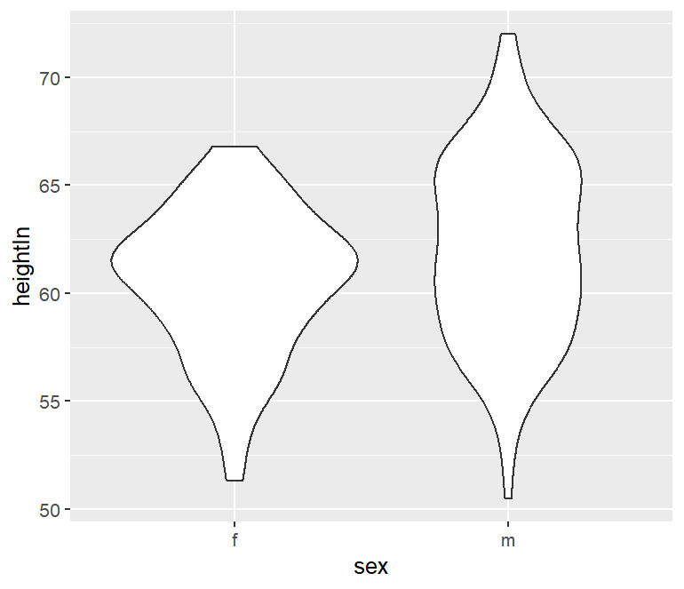
小提琴图

小提琴图可以观察到样本的分布情况，小提琴的宽度代表该数值位置样本数量的多少，越宽样本数量越多。小提琴图通过 geom_violin() 函数绘制。

1
2
3
4


library(gcookbook)
p <- ggplot(heightweight, aes(x = sex, y = heightIn))+
geom_violin()
p

设置箱线图和中位数点融合

1
2
3
4
5
6


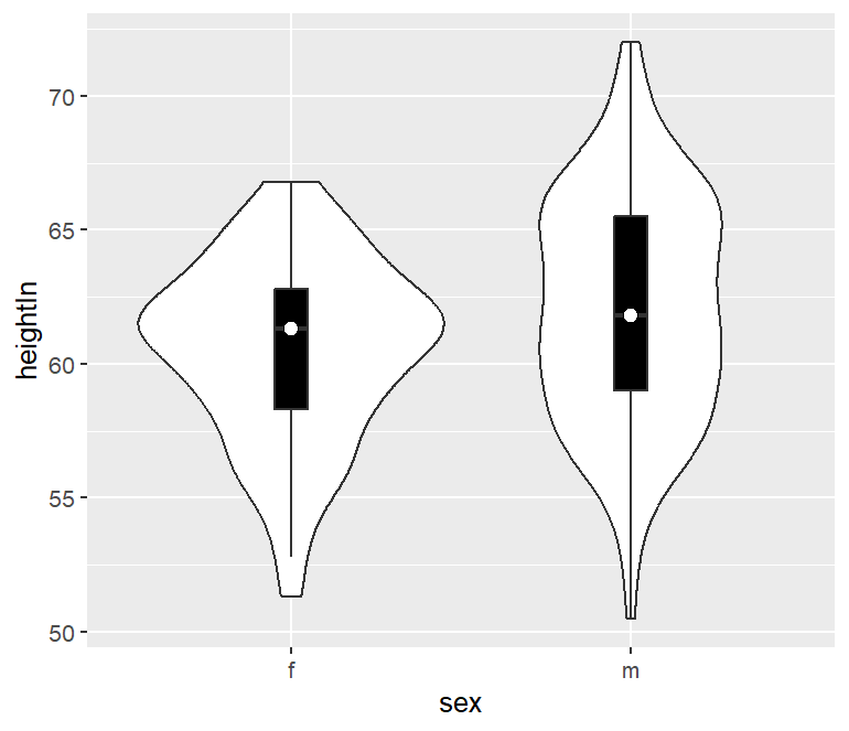
p <- ggplot(heightweight, aes(x = sex, y = heightIn))+
geom_violin()+
geom_boxplot(width = 0.1, fill = "black", outlier.color = NA)+
stat_summary(fun = median, geom = "point", fill = "white", shape = 21, size = 2.5)
# outlier.color = NA 不绘制离群点
p

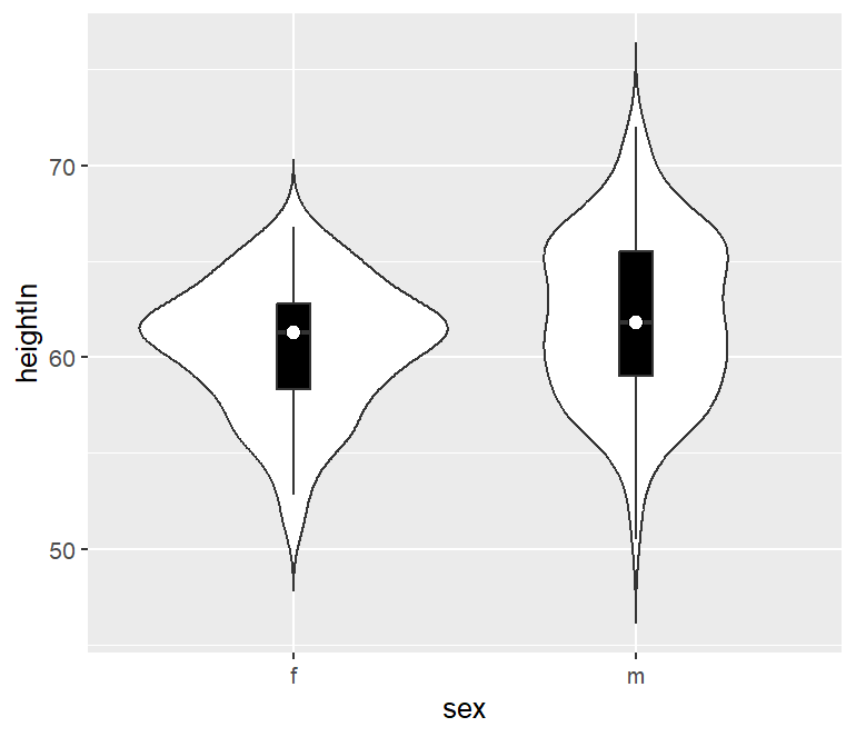
默认的小提琴图范围是从最小到最大数据值，可以通过设置 trim = FALSE 保留尾巴

1
2
3
4
5


p <- ggplot(heightweight, aes(x = sex, y = heightIn))+
geom_violin(trim = FALSE)+
geom_boxplot(width = 0.1, fill = "black", outlier.color = NA)+
stat_summary(fun = median, geom = "point", fill = "white", shape = 21, size = 2.5)
p

改变平滑量

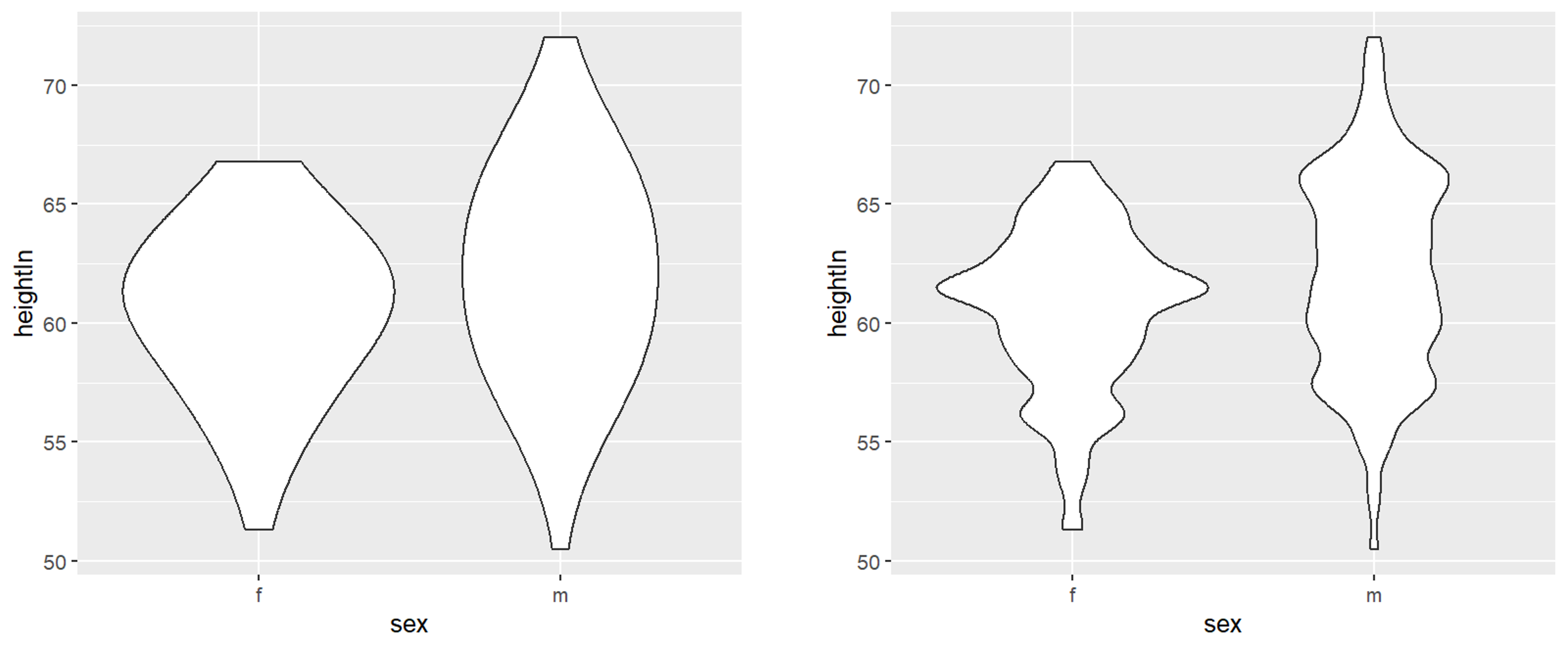
可以改变 adjust 参数来调整小提琴线轮廓的平滑程度

1
2
3
4
5
6
7
8
9


# 左图
p <- ggplot(heightweight, aes(x = sex, y = heightIn))+
geom_violin(adjust = 2)
p

# 右图
p <- ggplot(heightweight, aes(x = sex, y = heightIn))+
geom_violin(adjust = 0.5)
p

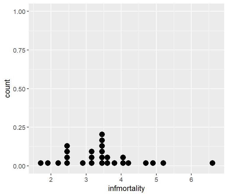
点阵图

又叫威尔金森点图（Wilkinson Dot Plot），是一种展示连续变量分布的点阵可视化，每个点代表 1 个观测样本，点堆叠的高度代表该区域样本频数，而非实际的 y 轴数值。选取 geom_dotplot() 进行绘图。

有点类似于 geom_histogram，两者都是把数据分箱看频数的分布，只不过直方图是柱状表示，而点阵图是点状表示。

 1
 2
 3
 4
 5
 6
 7
 8
 9
10


# 数据预处理
library(gcookbook)
library(tidyverse)
c2009 <- countries %>%
filter(Year == 2009 & healthexp > 2000)

# 绘图
p <- ggplot(c2009, aes(x = infmortality))+
geom_dotplot()
p

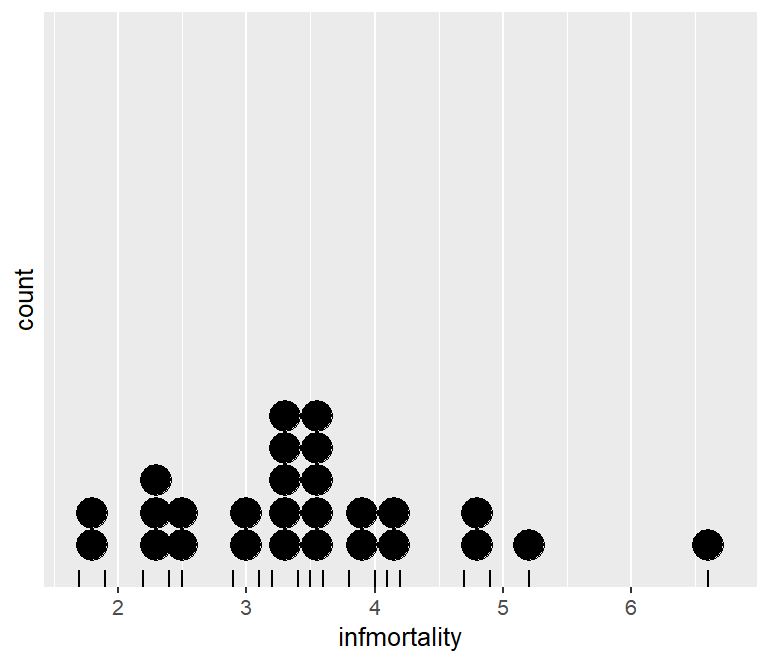
通过 binwidth 更改横轴每个箱的最大宽度，并美化点阵图

1
2
3
4
5
6


p <- ggplot(c2009, aes(x = infmortality))+
geom_dotplot(binwidth = .25)+
geom_rug()+
scale_y_continuous(breaks = NULL) # 删除 y 轴上全部数字刻度
theme(axis.title.y = element_blank()) # 删除 y 轴标签
p 

纵向分布多组点阵图

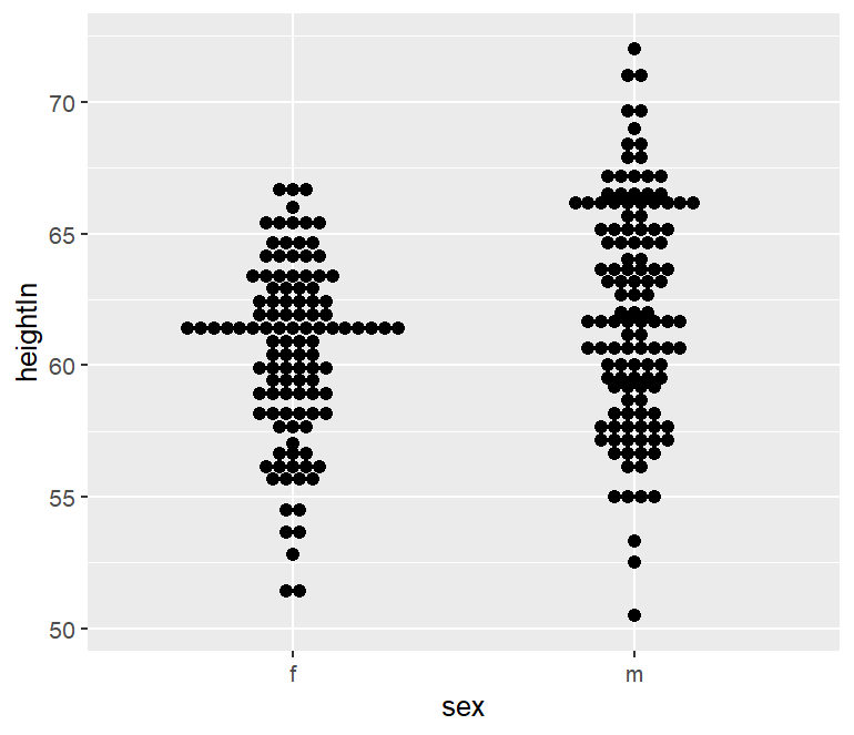
为了比较多个群，可以设置将点沿着 y 轴堆叠，并沿着 x 轴分组；可见下图其分布轮廓很像我们所作的小提琴图。

1
2
3


p <- ggplot(heightweight, aes(x = sex, y = heightIn))+
geom_dotplot(binaxis = "y", binwidth = .5, stackdir = "center")
p

叠加点阵图与箱线图

1
2
3
4


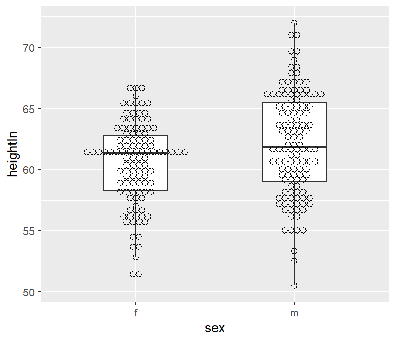
p <- ggplot(heightweight, aes(x = sex, y = heightIn))+
geom_boxplot(outlier.color = NA, width = .4)+
geom_dotplot(binaxis = "y", binwidth = .5, stackdir = "center", fill = NA)
p

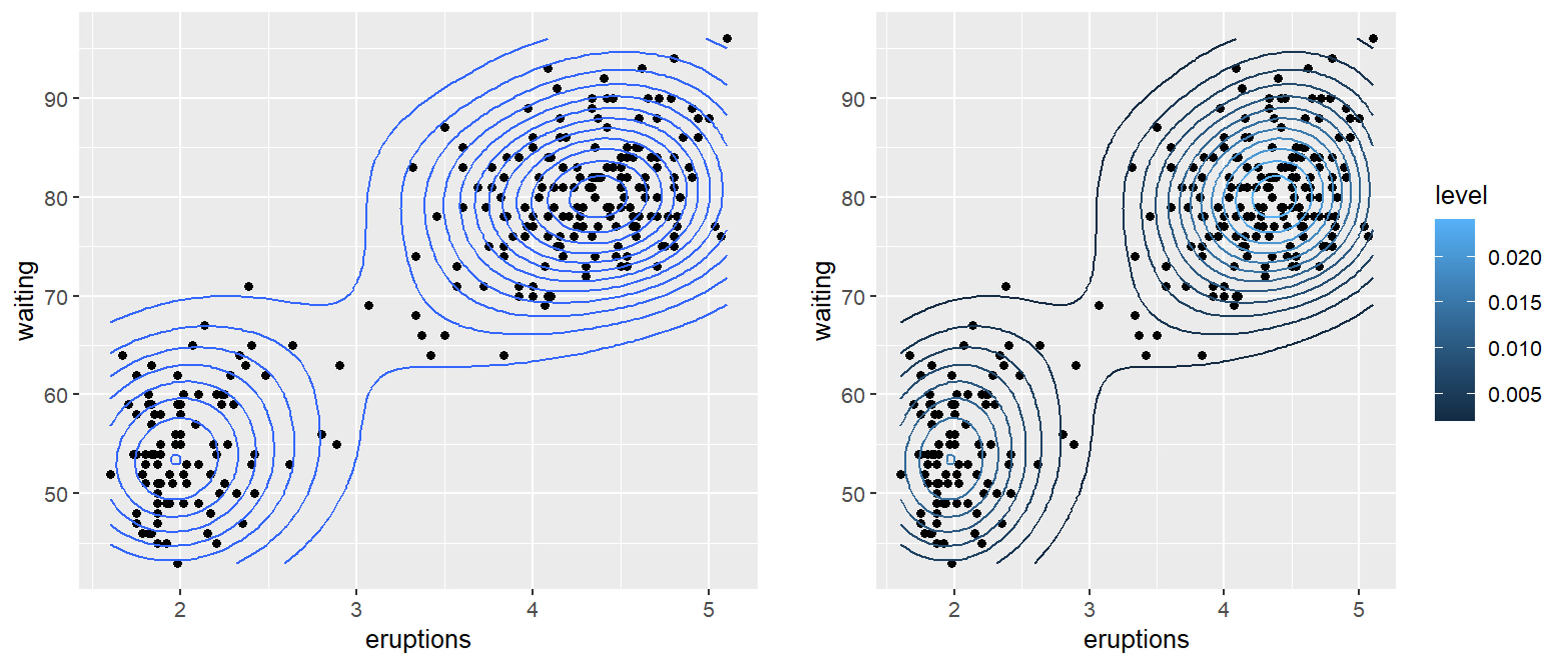
二维密度图

二维密度图可以同时处理 x、y 两个连续数值变量，估计二维平面上点的聚集程度，是二维版本核密度估计（KDE）；其解决了大量散点图重叠时样本密集的问题

 1
 2
 3
 4
 5
 6
 7
 8
 9
10


p <- ggplot(faithful, aes(x = eruptions, y = waiting))+
geom_point()+
stat_density2d()
p

p <- ggplot(faithful, aes(x = eruptions, y = waiting))+
geom_point()+
stat_density2d(aes(color = after_stat(level)))
# level 是绘制等高线后内部的派生变量，代表等高线的密度层级
p

填充

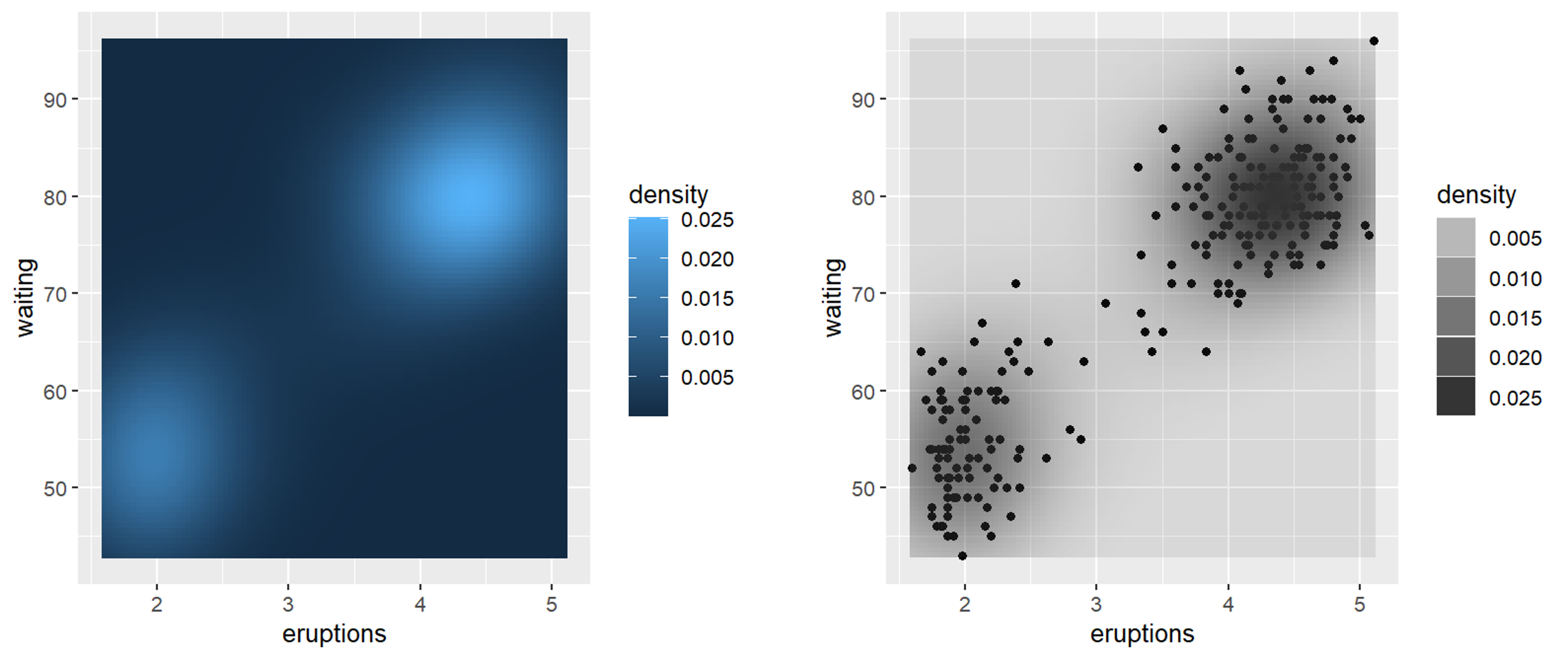
在 geom_density_2d() 中默认有 contour=TRUE 等高线层级，当关闭等高线层级后可以用原始二维核密度值来填充颜色表示密度

 1
 2
 3
 4
 5
 6
 7
 8
 9
10
11
12


p <- ggplot(faithful, aes(x = eruptions, y = waiting))+
stat_density2d(aes(fill = after_stat(density)), geom = "raster", contour = FALSE)
# 密度映射到 fill 填充颜色
# geom = "raster" 表示用 raster 光栅几何对象渲染密度网格
p

p <- ggplot(faithful, aes(x = eruptions, y = waiting))+
geom_point()+
stat_density2d(aes(alpha = after_stat(density)), geom = "tile", contour = FALSE)
# 密度映射到 alpha 透明度，底层叠原始点
# geom = "tile" 表示一个个矩形瓦片组成热力网格
p

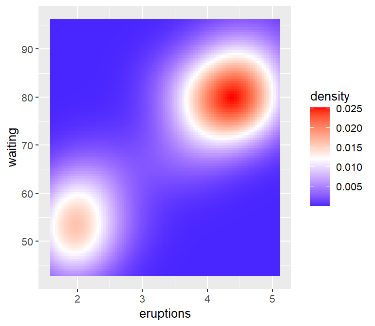
尝试把上面的默认颜色更改一下，好像也丑丑的……😫

1
2
3
4


p <- ggplot(faithful, aes(x = eruptions, y = waiting))+
stat_density2d(aes(fill = after_stat(density)), geom = "raster", contour = FALSE)+
scale_fill_gradient2(low = "blue", mid = "white", high = "red", midpoint = 0.012)
p

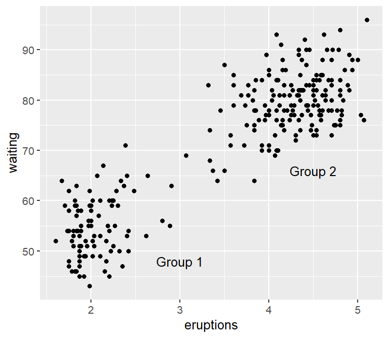
注释

通常情况下仅仅显示数据还不够，添加一些注释信息可让图片更直观、易解读。

1
2
3


annotate(geom, x, y, ...) 
# geom指定注释类型："text"、"segment"、"rect"、"point"、"arrow"
# x、y代表注释的坐标位置

文本注释

1
2
3
4
5


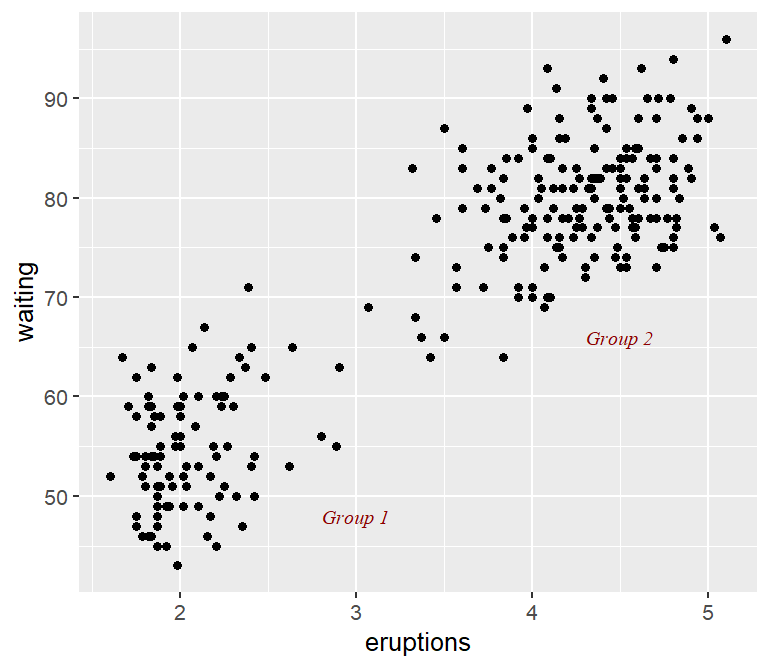
p <- ggplot(faithful, aes(x = eruptions, y = waiting)) +
geom_point()+
annotate("text", x = 3, y = 48, label = "Group 1")+
annotate("text", x = 4.5, y = 66, label = "Group 2")
p

更改 label 的样式

family 代表字体族，serif 是衬线字体（宋体类）；sans 为无衬线字体（黑体）

fonface 代表字体样式，italic 为斜体，plain 为普通，bold 为粗体，bold.italic 为粗斜体

1
2
3
4
5


p <- ggplot(faithful, aes(x = eruptions, y = waiting)) +
geom_point()+
annotate("text", x = 3, y = 48, label = "Group 1", family = "serif", fontface = "italic", color = "darkred", size = 3)+
annotate("text", x = 4.5, y = 66, label = "Group 2", family = "serif", fontface = "italic", color = "darkred", size = 3)
p

在特殊位置设置标签

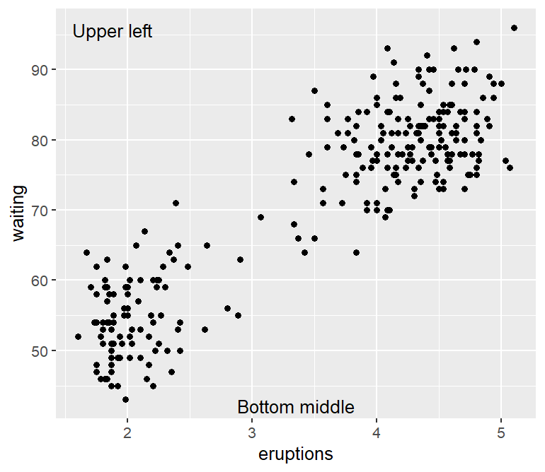
当位置参数 x 和 y 等于 Inf 时表示无穷大坐标，即可通过组合表示图片的四个角的位置

`hjust`	参考点为给定的 x 坐标，用于调整水平位置
`vjust`	参考点为给定的 y 坐标，用于调整垂直位置

1
2
3
4
5


p <- ggplot(faithful, aes(x = eruptions, y = waiting))+
geom_point()+
annotate("text", x = -Inf, y = Inf, label = "Upper left", hjust = -.2, vjust = 2)+
annotate("text", x = mean(range(faithful$eruptions)), y = -Inf, vjust = -0.4, label = "Bottom middle")
p

数学注释

 1
 2
 3
 4
 5
 6
 7
 8
 9
10
11
12
13
14


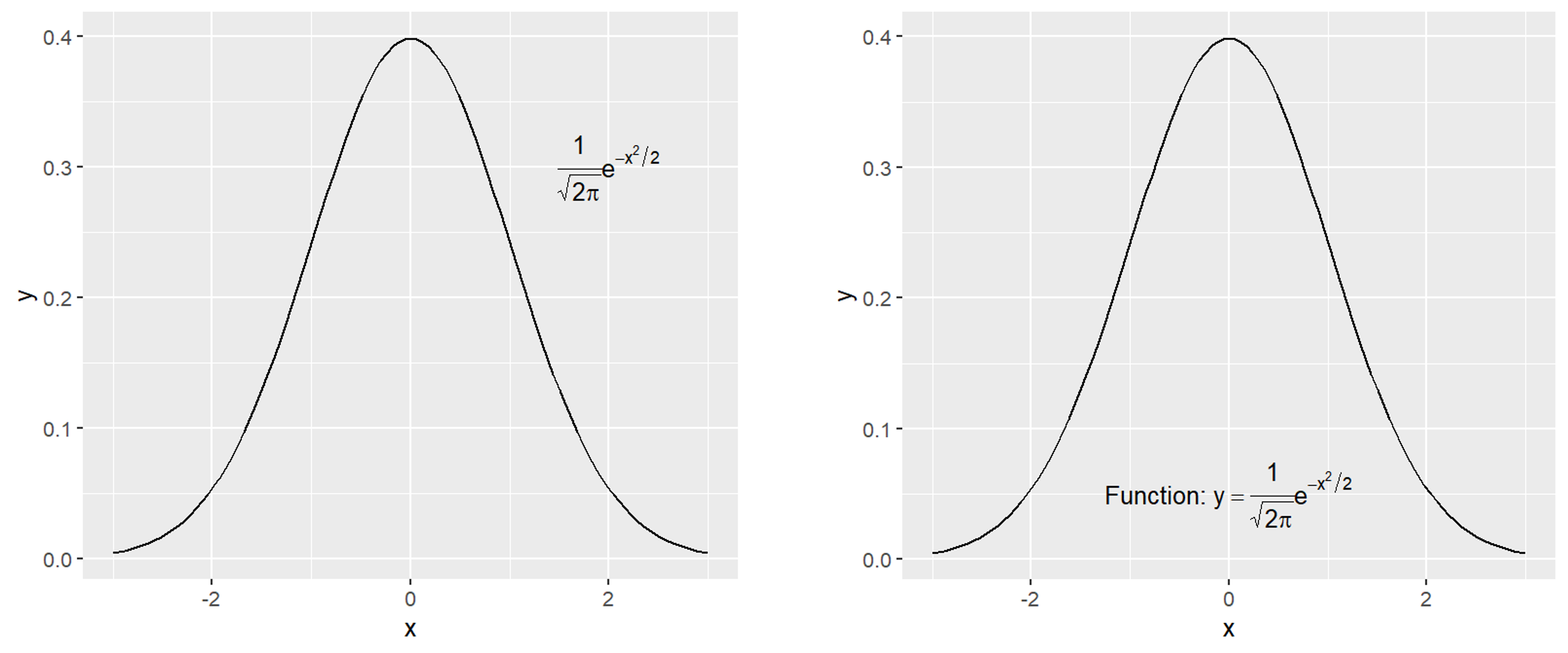
p <- ggplot(data.frame(x = c(-3, 3)), aes(x = x))+
stat_function(fun = dnorm)+
# stat_function() 属于 stat 统计层，会根据 dnorm 生成正态分布的 y 
annotate("text", x = 2, y = .3, parse = TRUE,
        label = "frac(1, sqrt(2 * pi)) * e ^ {-x^2 / 2}")
# parse = TRUE 使用的是 R 自带的 plotmath 数学语法
p

# 数学式子与文本内容混合需要使用''*标记明文部分
p <- ggplot(data.frame(x = c(-3, 3)), aes(x = x))+
stat_function(fun = dnorm)+
annotate("text", x = 0, y = .05, parse = TRUE,
        label = "'Function: '* y==frac(1, sqrt(2 * pi)) * e ^ {-x^2 / 2}")
p

线条

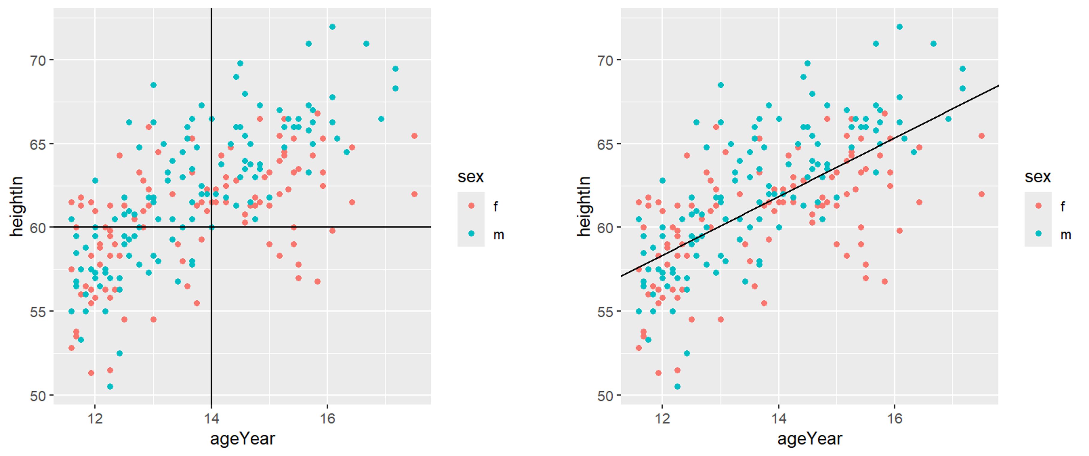
绘制线条主要可以使用 geom_hline()、geom_vline() 和 geom_abline() 来完成

`geom_hline()`	水平线
`geom_vline()`	垂直线
`geom_abline()`	一般直线

一般绘制

 1
 2
 3
 4
 5
 6
 7
 8
 9
10
11
12


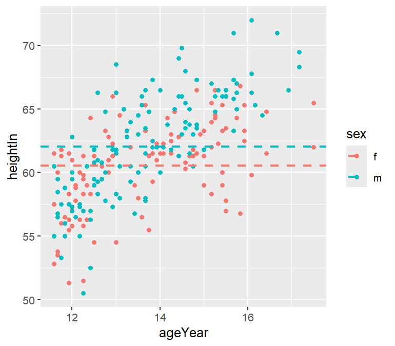
library(gcookbook)
p <- ggplot(heightweight, aes(x = ageYear, y = heightIn, color = sex))+
geom_point()+
geom_hline(yintercept = 60)+
geom_vline(xintercept = 14)
p

p <- ggplot(heightweight, aes(x = ageYear, y = heightIn, color = sex))+
geom_point()+
geom_abline(intercept = 37.4, slope = 1.75)
# intercept 和 slope 分别控制截距和斜率
p

绘制虚线

虚线绘制则增添 linetype 选取 "dashed"

 1
 2
 3
 4
 5
 6
 7
 8
 9
10


# 数据预处理
hw_means <- heightweight %>%
group_by(sex) %>%
summarise(heightIn = mean(heightIn))

# 绘制性别分类下平均体重虚线
p <- ggplot(heightweight, aes(x = ageYear, y = heightIn, color = sex))+
geom_point()+
geom_hline(data = hw_means, aes(yintercept = heightIn, colour = sex), linetype = "dashed", size = 1)
p

具有离散轴线的直线

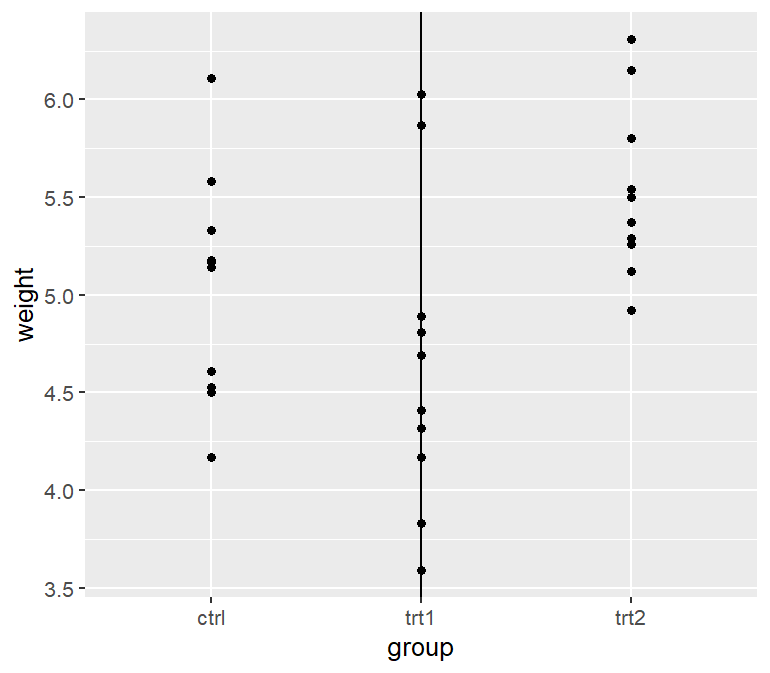
当存在某条轴的是离散的而非连续的，可用因子表示，第一层数值为 1，第二层值为 2，依此类推。

1
2
3
4
5
6


p <- ggplot(PlantGrowth, aes(x = group, y = weight))+
geom_point()+
geom_vline(xintercept = 2) # 第二个因子
p

# 等价于 geom_vline(xintercept = which(levels(PlantGrowth$group) == "trt1"))

线段与箭头

1
2
3
4
5
6
7
8
9


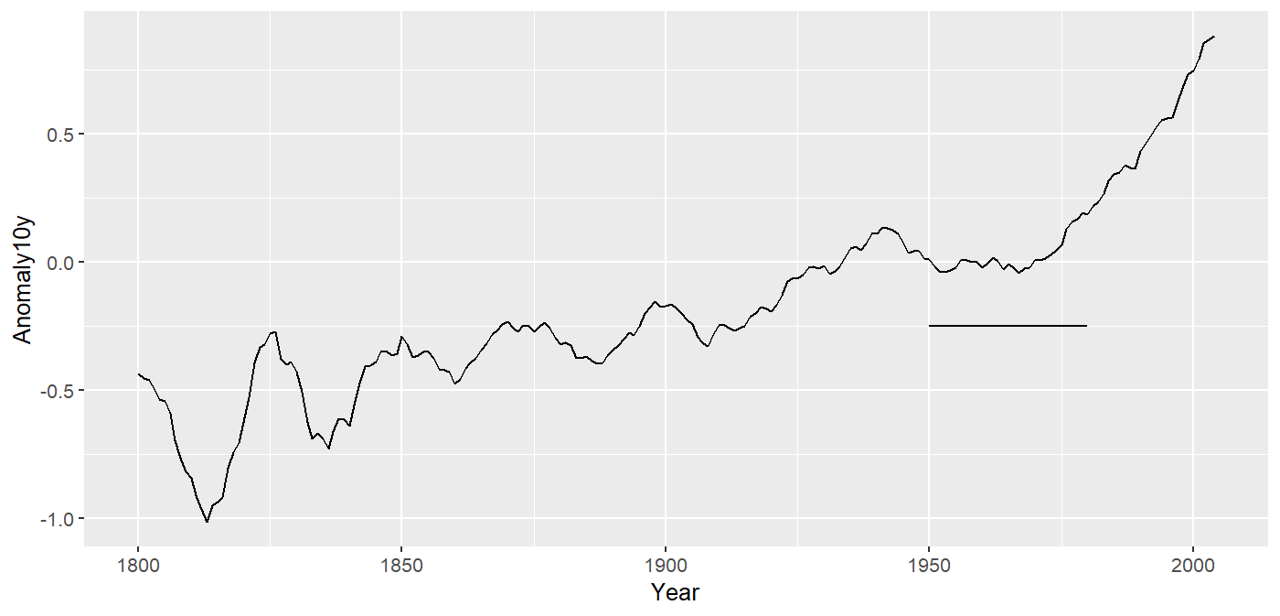
# 数据预处理
library(gcookbook)
cm <- climate %>%
filter(Source == "Berkeley")

p <- ggplot(cm, aes(x = Year, y = Anomaly10y))+
geom_line()+
annotate("segment", x = 1950, xend = 1980, y = -.25, yend = -.25)
p

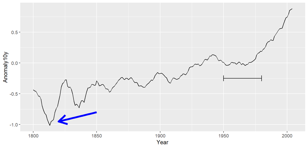
可以用网格给线段添加箭头或平端

1
2
3
4
5
6


p <- ggplot(cm, aes(x = Year, y = Anomaly10y))+
geom_line()+
annotate("segment", x = 1950, xend = 1980, y = -.25, yend = -.25, arrow = arrow(ends = "both", angle = 90, length = unit(.2, "cm")))+
annotate("segment", x = 1850, xend = 1820, y = -.8, yend = -.95, color = "blue", size = 2, arrow = arrow())
# 默认 arrow 角度为30，默认长度为 0.25 英寸
p

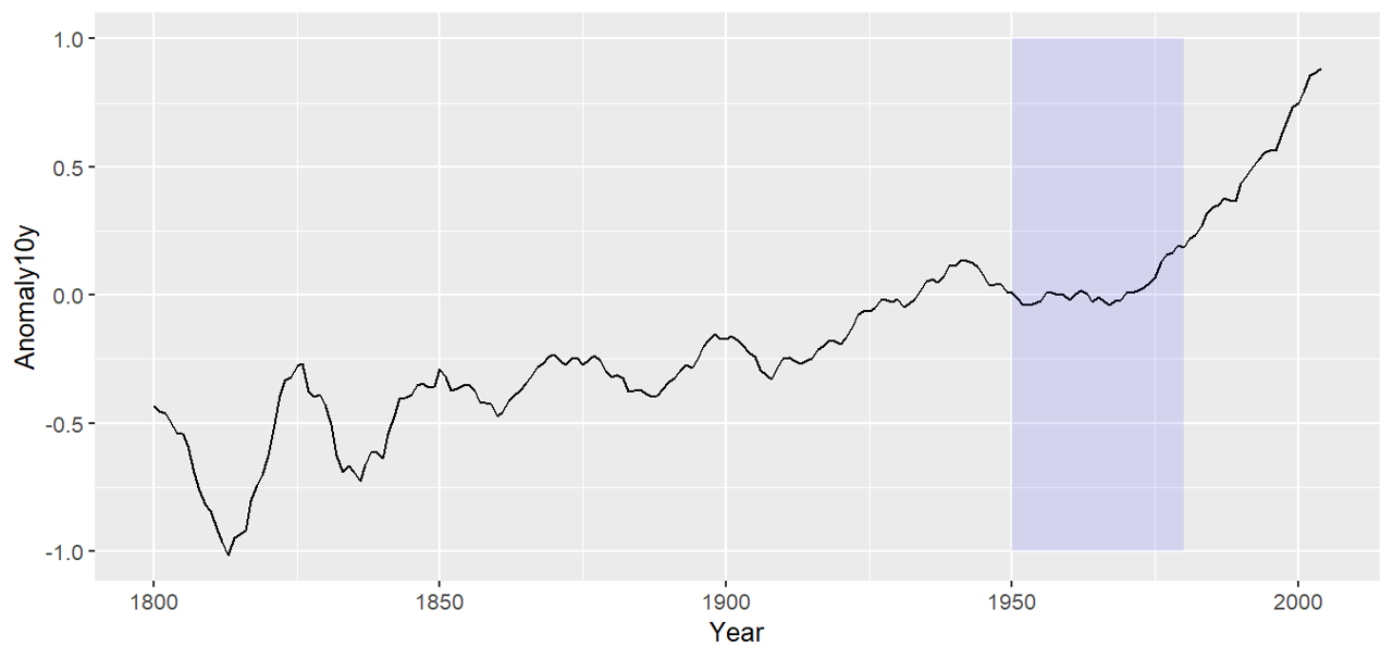
阴影

1
2
3
4
5
6


library(gcookbook)
p <- ggplot(filter(climate, Source == "Berkeley"), aes(x = Year, y = Anomaly10y))+
geom_line()+
annotate("rect", xmin = 1950, xmax = 1980, ymin = -1, ymax = 1, alpha = 0.1, fill = 'blue')
# 选择矩形注释
p

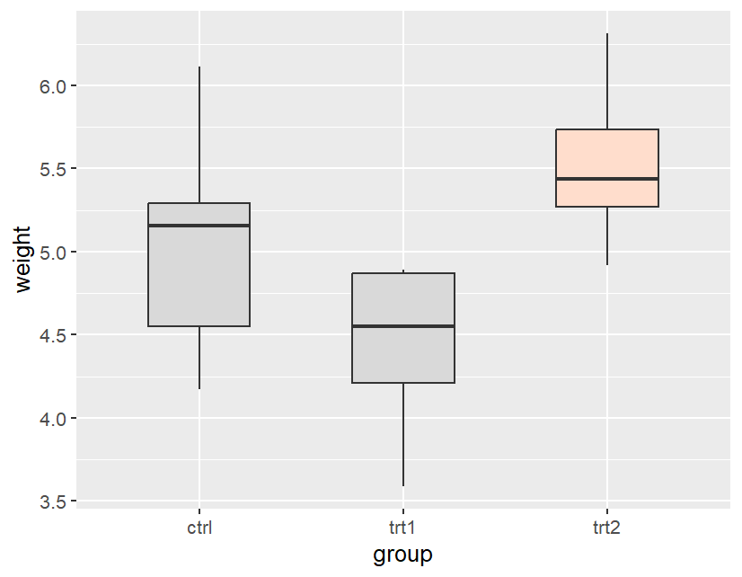
高亮

1
2
3
4
5
6
7
8
9


# 数据预处理
pg <- PlantGrowth %>%
mutate(hl = recode(group, "ctrl" = "no", "trt1" = "no", "trt2" = "yes"))
# 给数据框新增列

p <- ggplot(pg, aes(x = group, y = weight, fill =hl))+
geom_boxplot(width = .5, outliers = FALSE)+
scale_fill_manual(values = c("grey85", "#FFDDCC"), guide = FALSE)
p

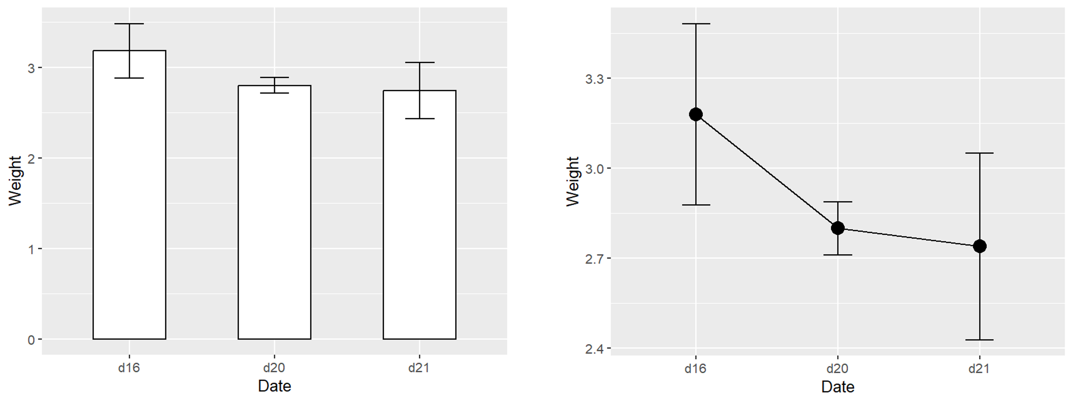
误差条

 1
 2
 3
 4
 5
 6
 7
 8
 9
10
11
12
13
14
15
16
17
18


# 数据预处理
library(gcookbook)
library(tidyverse)
ce <- cabbage_exp %>%
filter(Cultivar == "c39")

# geom_col() 柱状图
p <- ggplot(ce, aes(x = Date, y = Weight))+
geom_col(fill = "white", color = "black", width = .5)+
geom_errorbar(aes(ymin = Weight - se, ymax = Weight + se), width = .2)
p

# geom_line() 折线图
p <- ggplot(ce, aes(x = Date, y = Weight))+
geom_point(size = 4)+
geom_line(aes(group = 1))+
geom_errorbar(aes(ymin = Weight - se, ymax = Weight + se), width = .2)
p